In this tutorial you will learn how to implement Generative Adversarial Networks (GANs) using Keras and TensorFlow.

Generative Adversarial Networks were first introduced by Goodfellow et al. in their 2014 paper, Generative Adversarial Networks. These networks can be used to generate synthetic (i.e., fake) images that are perceptually near identical to their ground-truth authentic originals.

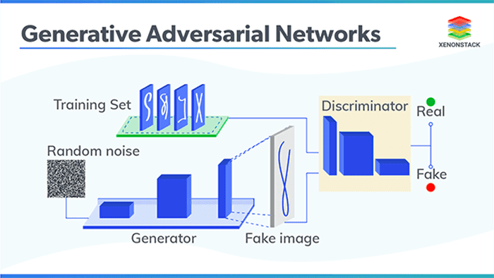
In order to generate synthetic images, we make use of two neural networks during training:

1. A generator that accepts an input vector of randomly generated noise and produces an output “imitation” image that looks similar, if not identical, to the authentic image
2. A discriminator or adversary that attempts to determine if a given image is an “authentic” or “fake”

By training these networks at the same time, one giving feedback to the other, we can learn to generate synthetic images.

Inside this tutorial we’ll be implementing a variation of Radford et al.’s paper, Unsupervised Representation Learning with Deep Convolutional Generative Adversarial Networks — or more simply, DCGANs.

As we’ll find out, training GANs can be a notoriously hard task, so we’ll implement a number of best practices recommended by both Radford et al. and Francois Chollet (creator of Keras and deep learning scientist at Google).

By the end of this tutorial, you’ll have a fully functioning GAN implementation.

To learn how to implement Generative Adversarial Networks (GANs) with Keras and TensorFlow, just keep reading.

Looking for the source code to this post?

Jump Right To The Downloads Section

GANs with Keras and TensorFlow

Note: This tutorial is a chapter from my book Deep Learning for Computer Vision with Python. If you enjoyed this post and would like to learn more about deep learning applied to computer vision, be sure to give my book a read — I have no doubt it will take you from deep learning beginner all the way to expert.

In the first part of this tutorial, we’ll discuss what Generative Adversarial Networks are, including how they are different from more “vanilla” network architectures you have seen before for classification and regression.

From there we’ll discuss the general GAN training process, including some guidelines and best practices you should follow when training your own GANs.

Next, we’ll review our directory structure for the project and then implement our GAN architecture using Keras and TensorFlow.

Once our GAN is implemented, we’ll train it on the Fashion MNIST dataset, thereby allowing us to generate fake/synthetic fashion apparel images.

Finally, we’ll wrap up this tutorial on Generative Adversarial Networks with a discussion of our results.

What are Generative Adversarial Networks (GANs)?

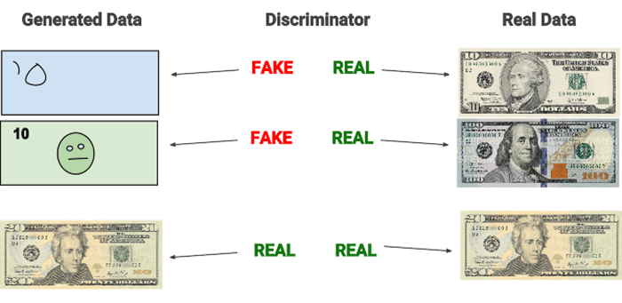
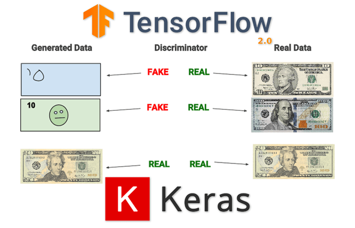
The quintessential explanation of GANs typically involves some variant of two people working in collusion to forge a set of documents, replicate a piece of artwork, or print counterfeit money — the counterfeit money printers is my personal favorite, and the one used by Chollet in his work.

In this example, we have two people:

1. Jack, the counterfeit printer (the generator)
2. Jason, an employee of the U.S. Treasury (which is responsible for printing money in the United States), who specializes in detecting counterfeit money (the discriminator)

Jack and Jason were childhood friends, both growing up without much money in the rough parts of Boston. After much hard work, Jason was awarded a college scholarship — Jack was not, and over time started to turn toward illegal ventures to make money (in this case, creating counterfeit money).

Jack knew he wasn’t very good at generating counterfeit money, but he felt that with the proper training, he could replicate bills that were passable in circulation.

One day, after a few too many pints at a local pub during the Thanksgiving holiday, Jason let it slip to Jack that he wasn’t happy with his job. He was underpaid. His boss was nasty and spiteful, often yelling and embarrassing Jason in front of other employees. Jason was even thinking of quitting.

Jack saw an opportunity to use Jason’s access at the U.S. Treasury to create an elaborate counterfeit printing scheme. Their conspiracy worked like this:

1. Jack, the counterfeit printer, would print fake bills and then mix both the fake bills and real money together, then show them to the expert, Jason.
2. Jason would sort through the bills, classifying each bill as “fake” or “authentic,” giving feedback to Jack along the way on how he could improve his counterfeit printing.

At first, Jack is doing a pretty poor job at printing counterfeit money. But over time, with Jason’s guidance, Jack eventually improves to the point where Jason is no longer able to spot the difference between the bills. By the end of this process, both Jack and Jason have stacks of counterfeit money that can fool most people.

The general GAN training procedure

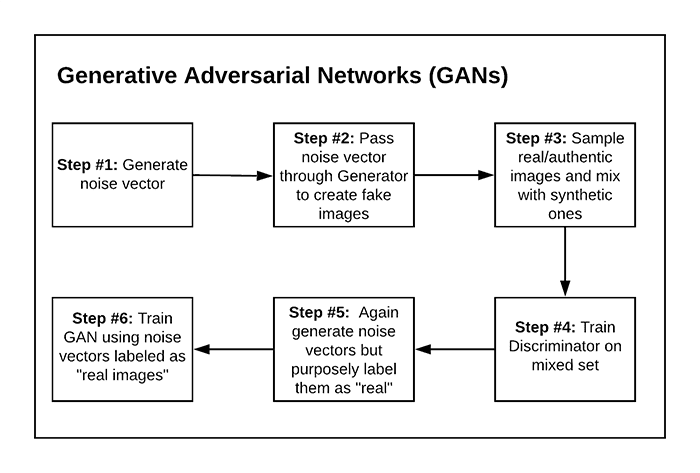
We’ve discussed what GANs are in terms of an analogy, but what is the actual procedure to train them? Most GANs are trained using a six-step process.

To start (Step 1), we randomly generate a vector (i.e., noise). We pass this noise through our generator, which generates an actual image (Step 2). We then sample authentic images from our training set and mix them with our synthetic images (Step 3).

The next step (Step 4) is to train our discriminator using this mixed set. The goal of the discriminator is to correctly label each image as “real” or “fake.”

Next, we’ll once again generate random noise, but this time we’ll purposely label each noise vector as a “real image” (Step 5). We’ll then train the GAN using the noise vectors and “real image” labels even though they are not actual real images (Step 6).

The reason this process works is due to the following:

1. We have frozen the weights of the discriminator at this stage, implying that the discriminator is not learning when we update the weights of the generator.
2. We’re trying to “fool” the discriminator into being unable to determine which images are real vs. synthetic. The feedback from the discriminator will allow the generator to learn how to produce more authentic images.

If you’re confused with this process, I would continue reading through our implementation covered later in this tutorial — seeing a GAN implemented in Python and then explained makes it easier to understand the process.

Guidelines and best practices when training GANs

GANs are notoriously hard to train due to an evolving loss landscape. At each iteration of our algorithm we are:

1. Generating random images and then training the discriminator to correctly distinguish the two
2. Generating additional synthetic images, but this time purposely trying to fool the discriminator
3. Updating the weights of the generator based on the feedback of the discriminator, thereby allowing us to generate more authentic images

From this process you’ll notice there are two losses we need to observe: one loss for the discriminator and a second loss for the generator. And since the loss landscape of the generator can be changed based on the feedback from the discriminator, we end up with a dynamic system.

When training GANs, our goal is not to seek a minimum loss value but instead to find some equilibrium between the two (Chollet 2017).

This concept of finding an equilibrium may make sense on paper, but once you try to implement and train your own GANs, you’ll find that this is a nontrivial process.

In their paper, Radford et al. recommend the following architecture guidelines for more stable GANs:

• Replace any pooling layers with strided convolutions (see this tutorial for more information on convolutions and strided convolutions).
• Use batch normalization in both the generator and discriminator.
• Remove fully-connected layers in deeper networks.
• Use ReLU in the generator except for the final layer, which will utilize tanh.
• Use Leaky ReLU in the discriminator.

In his book, Francois Chollet then provides additional recommendations on training GANs:

1. Sample random vectors from a normal distribution (i.e., Gaussian distribution) rather than a uniform distribution.
2. Add dropout to the discriminator.
3. Add noise to the class labels when training the discriminator.
4. To reduce checkerboard pixel artifacts in the output image, use a kernel size that is divisible by the stride when utilizing convolution or transposed convolution in both the generator and discriminator.
5. If your adversarial loss rises dramatically while your discriminator loss falls to zero, try reducing the learning rate of the discriminator and increasing the dropout of the discriminator.

Keep in mind that these are all just heuristics found to work in a number of situations — we’ll be using some of the techniques suggested by both Radford et al. and Chollet, but not all of them.

It is possible, and even probable, that the techniques listed here will not work on your GANs. Take the time now to set your expectations that you’ll likely be running orders of magnitude more experiments when tuning the hyperparameters of your GANs as compared to more basic classification or regression tasks.

Configuring your development environment to train GANs with Keras and TensorFlow

We’ll be using Keras and TensorFlow to implement and train our GANs.

I recommend you follow either of these two guides to install TensorFlow and Keras on your system:

• How to install TensorFlow 2.0 on Ubuntu
• How to install TensorFlow 2.0 on macOS

Either tutorial will help you configure your system with all the necessary software for this blog post in a convenient Python virtual environment.

Having problems configuring your development environment?

All that said, are you:

• Short on time?
• Learning on your employer’s administratively locked system?
• Wanting to skip the hassle of fighting with the command line, package managers, and virtual environments?
• Ready to run the code right now on your Windows, macOS, or Linux system?

Then join PyImageSearch Plus today!

Gain access to Jupyter Notebooks for this tutorial and other PyImageSearch guides that are pre-configured to run on Google Colab’s ecosystem right in your web browser! No installation required.

And best of all, these Jupyter Notebooks will run on Windows, macOS, and Linux!

Project structure

Now that we understand the fundamentals of Generative Adversarial Networks, let’s review our directory structure for the project.

Make sure you use the “Downloads” section of this tutorial to download the source code to our GAN project:

$ tree . --dirsfirst
.
├── output
│   ├── epoch_0001_output.png
│   ├── epoch_0001_step_00000.png
│   ├── epoch_0001_step_00025.png
...
│   ├── epoch_0050_step_00300.png
│   ├── epoch_0050_step_00400.png
│   └── epoch_0050_step_00500.png
├── pyimagesearch
│   ├── __init__.py
│   └── dcgan.py
└── dcgan_fashion_mnist.py

3 directories, 516 files

Implementing our “generator” with Keras and TensorFlow

Now that we’ve reviewed our project directory structure, let’s get started implementing our Generative Adversarial Network using Keras and TensorFlow.

Open up the dcgan.py file in our project directory structure, and let’s get started:

# import the necessary packages
from tensorflow.keras.models import Sequential
from tensorflow.keras.layers import BatchNormalization
from tensorflow.keras.layers import Conv2DTranspose
from tensorflow.keras.layers import Conv2D
from tensorflow.keras.layers import LeakyReLU
from tensorflow.keras.layers import Activation
from tensorflow.keras.layers import Flatten
from tensorflow.keras.layers import Dense
from tensorflow.keras.layers import Reshape

Lines 2-10 import our required Python packages. All of these classes should look fairly familiar to you, especially if you’ve read my Keras and TensorFlow tutorials or my book Deep Learning for Computer Vision with Python.

The only exception may be the Conv2DTranspose class. Transposed convolutional layers, sometimes referred to as fractionally-strided convolution or (incorrectly) deconvolution, are used when we need a transform going in the opposite direction of a normal convolution.

The generator of our GAN will accept an N dimensional input vector (i.e., a list of numbers, but a volume like an image) and then transform the N dimensional vector into an output image.

This process implies that we need to reshape and then upscale this vector into a volume as it passes through the network — to accomplish this reshaping and upscaling, we’ll need transposed convolution.

We can thus look at transposed convolution as the method to:

1. Accept an input volume from a previous layer in the network
2. Produce an output volume that is larger than the input volume
3. Maintain a connectivity pattern between the input and output

In essence our transposed convolution layer will reconstruct our target spatial resolution and perform a normal convolution operation, utilizing fancy zero-padding techniques to ensure our output spatial dimensions are met.

To learn more about transposed convolution, take a look at the Convolution arithmetic tutorial in the Theano documentation along with An introduction to different Types of Convolutions in Deep Learning By Paul-Louis Pröve.

Let’s now move into implementing our DCGAN class:

class DCGAN:
	@staticmethod
	def build_generator(dim, depth, channels=1, inputDim=100,
		outputDim=512):
		# initialize the model along with the input shape to be
		# "channels last" and the channels dimension itself
		model = Sequential()
		inputShape = (dim, dim, depth)
		chanDim = -1

The usage of these parameters will become more clear as we define the body of the network in the next code block.

Below we can find the body of our generator network:

		# first set of FC => RELU => BN layers
		model.add(Dense(input_dim=inputDim, units=outputDim))
		model.add(Activation("relu"))
		model.add(BatchNormalization())

		# second set of FC => RELU => BN layers, this time preparing
		# the number of FC nodes to be reshaped into a volume
		model.add(Dense(dim * dim * depth))
		model.add(Activation("relu"))
		model.add(BatchNormalization())

Lines 23-25 define our first set of FC => RELU => BN layers — applying batch normalization to stabilize GAN training is a guideline from Radford et al. (see the “Guidelines and best practices when training GANs” section above).

Notice how our FC layer will have an input dimension of inputDim (the randomly generated input vector) and then output dimensionality of outputDim. Typically outputDim will be larger than inputDim.

Lines 29-31 apply a second set of FC => RELU => BN layers, but this time we prepare the number of nodes in the FC layer to equal the number of units in inputShape (Line 29). Even though we are still utilizing a flattened representation, we need to ensure the output of this FC layer can be reshaped to our target volume sze (i.e., inputShape).

The actual reshaping takes place in the next code block:

		# reshape the output of the previous layer set, upsample +
		# apply a transposed convolution, RELU, and BN
		model.add(Reshape(inputShape))
		model.add(Conv2DTranspose(32, (5, 5), strides=(2, 2),
			padding="same"))
		model.add(Activation("relu"))
		model.add(BatchNormalization(axis=chanDim))

A call to Reshape while supplying the inputShape allows us to create a 3D volume from the fully-connected layer on Line 29. Again, this reshaping is only possible due to the fact that the number of output nodes in the FC layer matches the target inputShape.

We now reach an important guideline when training your own GANs:

1. To increase spatial resolution, use a transposed convolution with a stride > 1.
2. To create a deeper GAN without increasing spatial resolution, you can use either standard convolution or transposed convolution (but keep the stride equal to 1).

Here, our transposed convolution layer is learning 32 filters, each of which is 5×5, while applying a 2×2 stride — since our stride is > 1, we can increase our spatial resolution.

Let’s apply another transposed convolution:

		# apply another upsample and transposed convolution, but
		# this time output the TANH activation
		model.add(Conv2DTranspose(channels, (5, 5), strides=(2, 2),
			padding="same"))
		model.add(Activation("tanh"))

		# return the generator model
		return model

Lines 43 and 44 apply another transposed convolution, again increasing the spatial resolution, but taking care to ensure the number of filters learned is equal to the target number of channels (1 for grayscale and 3 for RGB).

We then apply a tanh activation function per the recommendation of Radford et al. The model is then returned to the calling function on Line 48.

Understanding the “generator” in our GAN

Assuming dim=7, depth=64, channels=1, inputDim=100, and outputDim=512 (as we will use when training our GAN on Fashion MNIST later in this tutorial), I have included the model summary below:

Model: "sequential"
_________________________________________________________________
Layer (type)                 Output Shape              Param #   
=================================================================
dense (Dense)                (None, 512)               51712     
_________________________________________________________________
activation (Activation)      (None, 512)               0         
_________________________________________________________________
batch_normalization (BatchNo (None, 512)               2048      
_________________________________________________________________
dense_1 (Dense)              (None, 3136)              1608768   
_________________________________________________________________
activation_1 (Activation)    (None, 3136)              0         
_________________________________________________________________
batch_normalization_1 (Batch (None, 3136)              12544     
_________________________________________________________________
reshape (Reshape)            (None, 7, 7, 64)          0         
_________________________________________________________________
conv2d_transpose (Conv2DTran (None, 14, 14, 32)        51232     
_________________________________________________________________
activation_2 (Activation)    (None, 14, 14, 32)        0         
_________________________________________________________________
batch_normalization_2 (Batch (None, 14, 14, 32)        128       
_________________________________________________________________
conv2d_transpose_1 (Conv2DTr (None, 28, 28, 1)         801       
_________________________________________________________________
activation_3 (Activation)    (None, 28, 28, 1)         0        
================================================================= 

Let’s break down what’s going on here.

Applying a transposed convolution with a 2×2 stride increases our spatial dimensions from 7×7 to 14×14.

A second transposed convolution (again, with a stride of 2×2) increases our spatial dimension resolution from 14×14 to 28×18 with a single channel, which is the exact dimensions of our input images in the Fashion MNIST dataset.

When implementing your own GANs, make sure the spatial dimensions of the output volume match the spatial dimensions of your input images. Use transposed convolution to increase the spatial dimensions of the volumes in the generator. I also recommend using model.summary() often to help you debug the spatial dimensions.

Implementing our “discriminator” with Keras and TensorFlow

The discriminator model is substantially more simplistic, similar to basic CNN classification architectures you may have read in my book or elsewhere on the PyImageSearch blog.

Keep in mind that while the generator is intended to create synthetic images, the discriminator is used to classify whether any given input image is real or fake.

Continuing our implementation of the DCGAN class in dcgan.py, let’s take a look at the discriminator now:

	@staticmethod
	def build_discriminator(width, height, depth, alpha=0.2):
		# initialize the model along with the input shape to be
		# "channels last"
		model = Sequential()
		inputShape = (height, width, depth)

		# first set of CONV => RELU layers
		model.add(Conv2D(32, (5, 5), padding="same", strides=(2, 2),
			input_shape=inputShape))
		model.add(LeakyReLU(alpha=alpha))

		# second set of CONV => RELU layers
		model.add(Conv2D(64, (5, 5), padding="same", strides=(2, 2)))
		model.add(LeakyReLU(alpha=alpha))

		# first (and only) set of FC => RELU layers
		model.add(Flatten())
		model.add(Dense(512))
		model.add(LeakyReLU(alpha=alpha))

		# sigmoid layer outputting a single value
		model.add(Dense(1))
		model.add(Activation("sigmoid"))

		# return the discriminator model
		return model

As we can see, this network is simple and straightforward. We first learn 32, 5×5 filters, followed by a second CONV layer, this one learning a total of 64, 5×5 filters. We only have a single FC layer here, this one with 512 nodes.

All activation layers utilize a Leaky ReLU activation to stabilize training, except for the final activation function which is sigmoid. We use a sigmoid here to capture the probability of whether the input image is real or synthetic.

Implementing our GAN training script

Now that we’ve implemented our DCGAN architecture, let’s train it on the Fashion MNIST dataset to generate fake apparel items. By the end of the training process, we will be unable to identify real images from synthetic ones.

Open up the dcgan_fashion_mnist.py file in our project directory structure, and let’s get to work:

# import the necessary packages
from pyimagesearch.dcgan import DCGAN
from tensorflow.keras.models import Model
from tensorflow.keras.layers import Input
from tensorflow.keras.optimizers import Adam
from tensorflow.keras.datasets import fashion_mnist
from sklearn.utils import shuffle
from imutils import build_montages
import numpy as np
import argparse
import cv2
import os

We start off by importing our required Python packages.

Let’s move to parsing our command line arguments:

# construct the argument parse and parse the arguments
ap = argparse.ArgumentParser()
ap.add_argument("-o", "--output", required=True,
	help="path to output directory")
ap.add_argument("-e", "--epochs", type=int, default=50,
	help="# epochs to train for")
ap.add_argument("-b", "--batch-size", type=int, default=128,
	help="batch size for training")
args = vars(ap.parse_args())

We require only a single command line argument for this script, --output, which is the path to the output directory where we’ll store montages of generated images (thereby allowing us to visualize the GAN training process).

We can also (optionally) supply --epochs, the total number of epochs to train for, and --batch-size, used to control the batch size when training.

Let’s now take care of a few important initializations:

# store the epochs and batch size in convenience variables, then
# initialize our learning rate
NUM_EPOCHS = args["epochs"]
BATCH_SIZE = args["batch_size"]
INIT_LR = 2e-4

We store both the number of epochs and batch size in convenience variables on Lines 26 and 27.

We also initialize our initial learning rate (INIT_LR) on Line 28. This value was empirically tuned through a number of experiments and trial and error. If you choose to apply this GAN implementation to your own dataset, you may need to tune this learning rate.

We can now load the Fashion MNIST dataset from disk:

# load the Fashion MNIST dataset and stack the training and testing
# data points so we have additional training data
print("[INFO] loading MNIST dataset...")
((trainX, _), (testX, _)) = fashion_mnist.load_data()
trainImages = np.concatenate([trainX, testX])

# add in an extra dimension for the channel and scale the images
# into the range [-1, 1] (which is the range of the tanh
# function)
trainImages = np.expand_dims(trainImages, axis=-1)
trainImages = (trainImages.astype("float") - 127.5) / 127.5

Line 33 loads the Fashion MNIST dataset from disk. We ignore class labels here, since we do not need them — we are only interested in the actual pixel data.

Furthermore, there is no concept of a “test set” for GANs. Our goal when training a GAN isn’t minimal loss or high accuracy. Instead, we seek an equilibrium between the generator and the discriminator.

To help us obtain this equilibrium, we combine both the training and testing images (Line 34) to give us additional training data.

Lines 39 and 40 prepare our data for training by scaling the pixel intensities to the range [0, 1], the output range of the tanh activation function.

Let’s now initialize our generator and discriminator:

# build the generator
print("[INFO] building generator...")
gen = DCGAN.build_generator(7, 64, channels=1)

# build the discriminator
print("[INFO] building discriminator...")
disc = DCGAN.build_discriminator(28, 28, 1)
discOpt = Adam(lr=INIT_LR, beta_1=0.5, decay=INIT_LR / NUM_EPOCHS)
disc.compile(loss="binary_crossentropy", optimizer=discOpt)

Line 44 initializes the generator that will transform the input random vector to a volume of shape 7x7x64-channel map.

Lines 48-50 build the discriminator and then compile it using the Adam optimizer with binary cross-entropy loss.

Keep in mind that we are using binary cross-entropy here, as our discriminator has a sigmoid activation function that will return a probability indicating whether the input image is real vs. fake. Since there are only two “class labels” (real vs. synthetic), we use binary cross-entropy.

The learning rate and beta value for the Adam optimizer were experimentally tuned. I’ve found that a lower learning rate and beta value for the Adam optimizer improves GAN training on the Fashion MNIST dataset. Applying learning rate decay helps stabilize training as well.

Given both the generator and discriminator, we can build our GAN:

# build the adversarial model by first setting the discriminator to
# *not* be trainable, then combine the generator and discriminator
# together
print("[INFO] building GAN...")
disc.trainable = False
ganInput = Input(shape=(100,))
ganOutput = disc(gen(ganInput))
gan = Model(ganInput, ganOutput)

# compile the GAN
ganOpt = Adam(lr=INIT_LR, beta_1=0.5, decay=INIT_LR / NUM_EPOCHS)
gan.compile(loss="binary_crossentropy", optimizer=discOpt)

The actual GAN consists of both the generator and the discriminator; however, we first need to freeze the discriminator weights (Line 56) before we combine the models to form our Generative Adversarial Network (Lines 57-59).

Here we can see that the input to the gan will take a random vector that is 100-d. This value will be passed through the generator first, the output of which will go to the discriminator — we call this “model composition,” similar to “function composition” we learned about back in algebra class.

The discriminator weights are frozen at this point so the feedback from the discriminator will enable the generator to learn how to generate better synthetic images.

Lines 62 and 63 compile the gan. I again use the Adam optimizer with the same hyperparameters as the optimizer for the discriminator — this process worked for the purposes of these experiments, but you may need to tune these values on your own datasets and models.

Additionally, I’ve often found that setting the learning rate of the GAN to be half that of the discriminator is often a good starting point.

Throughout the training process we’ll want to see how our GAN evolves to construct synthetic images from random noise. To accomplish this task, we’ll need to generate some benchmark random noise used to visualize the training process:

# randomly generate some benchmark noise so we can consistently
# visualize how the generative modeling is learning
print("[INFO] starting training...")
benchmarkNoise = np.random.uniform(-1, 1, size=(256, 100))

# loop over the epochs
for epoch in range(0, NUM_EPOCHS):
	# show epoch information and compute the number of batches per
	# epoch
	print("[INFO] starting epoch {} of {}...".format(epoch + 1,
		NUM_EPOCHS))
	batchesPerEpoch = int(trainImages.shape[0] / BATCH_SIZE)

	# loop over the batches
	for i in range(0, batchesPerEpoch):
		# initialize an (empty) output path
		p = None

		# select the next batch of images, then randomly generate
		# noise for the generator to predict on
		imageBatch = trainImages[i * BATCH_SIZE:(i + 1) * BATCH_SIZE]
		noise = np.random.uniform(-1, 1, size=(BATCH_SIZE, 100))

Line 68 generates our benchmarkNoise. Notice that the benchmarkNoise is generated from a uniform distribution in the range [-1, 1], the same range as our tanh activation function. Line 68 indicates that we’ll be generating 256 synthetic images, where each input starts as a 100-d vector.

Starting on Line 71 we loop over our desired number of epochs. Line 76 computes the number of batches per epoch by dividing the number of training images by the supplied batch size.

We then loop over each batch on Line 79.

		# generate images using the noise + generator model
		genImages = gen.predict(noise, verbose=0)

		# concatenate the *actual* images and the *generated* images,
		# construct class labels for the discriminator, and shuffle
		# the data
		X = np.concatenate((imageBatch, genImages))
		y = ([1] * BATCH_SIZE) + ([0] * BATCH_SIZE)
		y = np.reshape(y, (-1,))
		(X, y) = shuffle(X, y)

		# train the discriminator on the data
		discLoss = disc.train_on_batch(X, y)

Line 89 takes our input noise and then generates synthetic apparel images (genImages).

Given our generated images, we need to train the discriminator to recognize the difference between real and synthetic images.

To accomplish this task, Line 94 concatenates the current imageBatch and the synthetic genImages together.

We then need to build our class labels on Line 95 — each real image will have a class label of 1, while every fake image will be labeled 0.

The concatenated training data is then jointly shuffled on Line 97 so our real and fake images do not sequentially follow each other one-by-one (which would cause problems during our gradient update phase).

Additionally, I have found this shuffling process improves the stability of discriminator training.

Line 100 trains the discriminator on the current (shuffled) batch.

The final step in our training process is to train the gan itself:

		# let's now train our generator via the adversarial model by
		# (1) generating random noise and (2) training the generator
		# with the discriminator weights frozen
		noise = np.random.uniform(-1, 1, (BATCH_SIZE, 100))
		fakeLabels = [1] * BATCH_SIZE
		fakeLabels = np.reshape(fakeLabels, (-1,))
		ganLoss = gan.train_on_batch(noise, fakeLabels)

We first generate a total of BATCH_SIZE random vectors. However, unlike in our previous code block, where we were nice enough to tell our discriminator what is real vs. fake, we’re now going to attempt to trick the discriminator by labeling the random noise as real images.

The feedback from the discriminator enables us to actually train the generator (keeping in mind that the discriminator weights are frozen for this operation).

Not only is looking at the loss values important when training a GAN, but you also need to examine the output of the gan on your benchmarkNoise:

		# check to see if this is the end of an epoch, and if so,
		# initialize the output path
		if i == batchesPerEpoch - 1:
			p = [args["output"], "epoch_{}_output.png".format(
				str(epoch + 1).zfill(4))]

		# otherwise, check to see if we should visualize the current
		# batch for the epoch
		else:
			# create more visualizations early in the training
			# process
			if epoch < 10 and i % 25 == 0:
				p = [args["output"], "epoch_{}_step_{}.png".format(
					str(epoch + 1).zfill(4), str(i).zfill(5))]

			# visualizations later in the training process are less
			# interesting
			elif epoch >= 10 and i % 100 == 0:
				p = [args["output"], "epoch_{}_step_{}.png".format(
					str(epoch + 1).zfill(4), str(i).zfill(5))]

If we have reached the end of the epoch, we’ll build the path, p, to our output visualization (Lines 112-114).

Otherwise, I find it helpful to visually inspect the output of our GAN with more frequency in earlier steps rather than later ones (Lines 118-129).

The output visualization will be totally random salt and pepper noise at the beginning but should quickly start to develop characteristics of the input data. These characteristics may not look real, but the evolving attributes will demonstrate to you that the network is actually learning.

If your output visualizations are still salt and pepper noise after 5-10 epochs, it may be a sign that you need to tune your hyperparameters, potentially including the model architecture definition itself.

Our final code block handles writing the synthetic image visualization to disk:

		# check to see if we should visualize the output of the
		# generator model on our benchmark data
		if p is not None:
			# show loss information
			print("[INFO] Step {}_{}: discriminator_loss={:.6f}, "
				"adversarial_loss={:.6f}".format(epoch + 1, i,
					discLoss, ganLoss))

			# make predictions on the benchmark noise, scale it back
			# to the range [0, 255], and generate the montage
			images = gen.predict(benchmarkNoise)
			images = ((images * 127.5) + 127.5).astype("uint8")
			images = np.repeat(images, 3, axis=-1)
			vis = build_montages(images, (28, 28), (16, 16))[0]

			# write the visualization to disk
			p = os.path.sep.join(p)
			cv2.imwrite(p, vis)

Line 141 uses our generator to generate images from our benchmarkNoise. We then scale our image data back from the range [-1, 1] (the boundaries of the tanh activation function) to the range [0, 255] (Line 142).

Since we are generating single-channel images, we repeat the grayscale representation of the image three times to construct a 3-channel RGB image (Line 143).

The build_montages function generates a 16×16 grid, with a 28×28 image in each vector. The montage is then written to disk on Line 148.

Training our GAN with Keras and TensorFlow

To train our GAN on the Fashion MNIST dataset, make sure you use the “Downloads” section of this tutorial to download the source code.

From there, open up a terminal, and execute the following command:

$ python dcgan_fashion_mnist.py --output output
[INFO] loading MNIST dataset...
[INFO] building generator...
[INFO] building discriminator...
[INFO] building GAN...
[INFO] starting training...
[INFO] starting epoch 1 of 50...
[INFO] Step 1_0: discriminator_loss=0.683195, adversarial_loss=0.577937
[INFO] Step 1_25: discriminator_loss=0.091885, adversarial_loss=0.007404
[INFO] Step 1_50: discriminator_loss=0.000986, adversarial_loss=0.000562
...
[INFO] starting epoch 50 of 50...
[INFO] Step 50_0: discriminator_loss=0.472731, adversarial_loss=1.194858
[INFO] Step 50_100: discriminator_loss=0.526521, adversarial_loss=1.816754
[INFO] Step 50_200: discriminator_loss=0.500521, adversarial_loss=1.561429
[INFO] Step 50_300: discriminator_loss=0.495300, adversarial_loss=0.963850
[INFO] Step 50_400: discriminator_loss=0.512699, adversarial_loss=0.858868
[INFO] Step 50_500: discriminator_loss=0.493293, adversarial_loss=0.963694
[INFO] Step 50_545: discriminator_loss=0.455144, adversarial_loss=1.128864

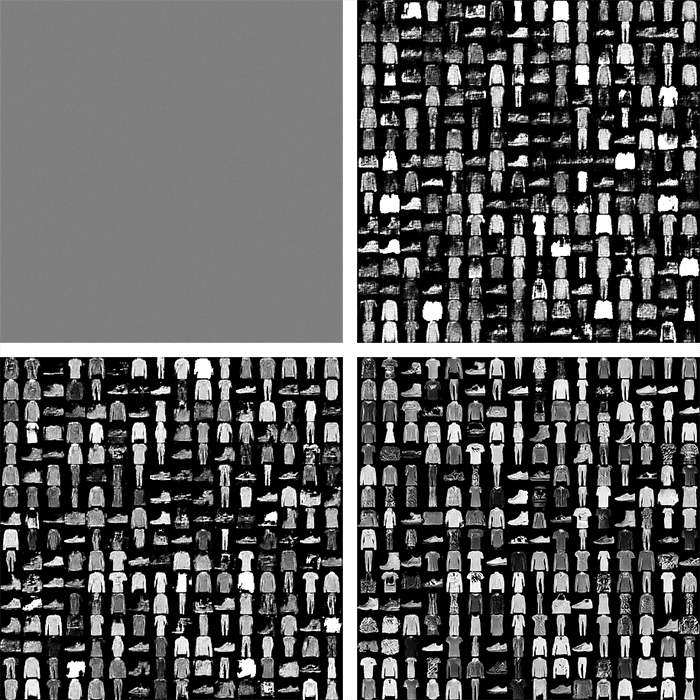
Figure 5 shows our random noise vectors (i.e., benchmarkNoise during different moments of training):

• The top-left contains 256 (in an 8×8 grid) of our initial random noise vectors before even starting to train the GAN. We can clearly see there is no pattern in this noise. No fashion items have been learned by the GAN.
• However, by the end of the second epoch (top-right), apparel-like structures are starting to appear.
• By the end of the fifth epoch (bottom-left), the fashion items are significantly more clear.
• And by the time we reach the end of the 50th epoch (bottom-right), our fashion items look authentic.

Again, it’s important to understand that these fashion items are generated from random noise input vectors — they are totally synthetic images!

What’s next?

As stated at the beginning of this tutorial, the majority of this blog post comes from my book, Deep Learning for Computer Vision with Python (DL4CV).

If you have not yet had the opportunity to join the DL4CV course, I hope you enjoyed your sneak preview! Not only are the fundamentals of neural networks reviewed, covered, and practiced throughout the DL4CV course, but so are more complex models and architectures, including GANs, super resolution, object detection (Faster R-CNN, SSDs, RetinaNet) and instance segmentation (Mask R-CNN).

Whether you are a professional, practitioner, or hobbyist – I crafted my Deep Learning for Computer Vision with Python book so that it perfectly blends theory with code implementation, ensuring you can master:

• Deep learning fundamentals and theory without unnecessary mathematical fluff. I present the basic equations and back them up with code walkthroughs that you can implement and easily understand. You don’t need a degree in advanced mathematics to understand this book.
• How to implement your own custom neural network architectures. Not only will you learn how to implement state-of-the-art architectures, including ResNet, SqueezeNet, etc., but you’ll also learn how to create your own custom CNNs.
• How to train CNNs on your own datasets. Most deep learning tutorials don’t teach you how to work with your own custom datasets. Mine do. You’ll be training CNNs on your own datasets in no time.
• Object detection (Faster R-CNNs, Single Shot Detectors, and RetinaNet) and instance segmentation (Mask R-CNN). Use these chapters to create your own custom object detectors and segmentation networks.

You’ll also find answers and proven code recipes to:

• Create and prepare your own custom image datasets for image classification, object detection, and segmentation
• Work through hands-on tutorials (with lots of code) that not only show you the algorithms behind deep learning for computer vision but their implementations as well
• Put my tips, suggestions, and best practices into action, ensuring you maximize the accuracy of your models

Beginners and experts alike tend to resonate with my no-nonsense teaching style and high-quality content.

If you’re on the fence about taking the next step in your computer vision, deep learning, and artificial intelligence education, be sure to read my Student Success Stories. My readers have gone on to excel in their careers — you can too!

If you’re ready to begin, purchase your copy here today. And if you aren’t convinced yet, I’d be happy to send you the full table of contents + sample chapters — simply click here. You can also browse my library of other book and course offerings.

Summary

In this tutorial we discussed Generative Adversarial Networks (GANs). We learned that GANs actually consist of two networks:

1. A generator that is responsible for generating fake images
2. A discriminator that tries to spot the synthetic images from the authentic ones

By training both of these networks at the same time, we can learn to generate very realistic output images.

We then implemented Deep Convolutional Adversarial Networks (DCGANS), a variation of Goodfellow et al.’s original GAN implementation.

Using our DCGAN implementation, we trained both the generator and discriminator on the Fashion MNIST dataset, resulting in output images of fashion items that:

1. Are not part of the training set and are complete synthetic
2. Look nearly identical to and indistinguishable from any image in the Fashion MNIST dataset

The problem is that training GANs can be extremely challenging, more so than any other architecture or method we have discussed on the PyImageSearch blog.

The reason GANs are notoriously hard to train is due to the evolving loss landscape — with every step, our loss landscape changes slightly and is thus ever-evolving.

The evolving loss landscape is in stark contrast to other classification or regression tasks where the loss landscape is “fixed” and nonmoving.

When training your own GANs, you’ll undoubtedly have to carefully tune your model architecture and associated hyperparameters — be sure to refer to the “Guidelines and best practices when training GANs” section at the top of this tutorial to help you tune your hyperparameters and run your own GAN experiments.

To download the source code to this post (and be notified when future tutorials are published here on PyImageSearch), simply enter your email address in the form below!

Download the Source Code and FREE 17-page Resource Guide

Enter your email address below to get a .zip of the code and a FREE 17-page Resource Guide on Computer Vision, OpenCV, and Deep Learning. Inside you'll find my hand-picked tutorials, books, courses, and libraries to help you master CV and DL!

Download the code!

Website

The post GANs with Keras and TensorFlow appeared first on PyImageSearch.

In this tutorial you will learn how to build image pairs for training siamese networks. We’ll implement our image pair generator using Python so that you can use the same code, regardless of whether you’re using TensorFlow, Keras, PyTorch, etc.

This tutorial is part one in an introduction to siamese networks:

• Part #1: Building image pairs for siamese networks with Python (today’s post)
• Part #2: Training siamese networks with Keras, TensorFlow, and Deep Learning (next week’s tutorial)
• Part #3: Comparing images using siamese networks (tutorial two weeks from now)

Siamese networks are incredibly powerful networks, responsible for significant increases in face recognition, signature verification, and prescription pill identification applications (just to name a few).

In fact, if you’ve followed my tutorial on OpenCV Face Recognition or Face recognition with OpenCV, Python and deep learning, you will see that the deep learning models used in these posts were siamese networks!

Deep learning models such as FaceNet, VGGFace, and dlib’s ResNet face recognition model are all examples of siamese networks.

And furthermore, siamese networks make more advanced training procedures like one-shot learning and few-shot learning possible — in comparison to other deep learning architectures, siamese networks require very few training examples, to be effective.

Today we’re going to:

• Review the basics of siamese networks
• Discuss the concept of image pairs
• See how we use image pairs to train a siamese network
• Implement Python code to generate image pairs for siamese networks

Next week I’ll show you how to implement and train your own siamese network. Eventually, we’ll build up to the concept of image triplets and how we can use triplet loss and contrastive loss to train better, more accurate siamese networks.

But for now, let’s understand image pairs, a fundamental requirement when implementing basic siamese networks.

To learn how to build image pairs for siamese networks, just keep reading.

Looking for the source code to this post?

Jump Right To The Downloads Section

Building image pairs for siamese networks with Python

In the first part of this tutorial, I’ll provide a high-level overview of siamese networks, including:

• What they are
• Why we use them
• When to use them
• How they are trained

We’ll then discuss the concept of “image pairs” in siamese networks, including why constructing image pairs is a requirement when training siamese networks.

From there we’ll review our project directory structure and then implement a Python script to generate image pairs. You can use this image pair generation function in your own siamese network training procedures, regardless of whether you are using Keras, TensorFlow, PyTorch, etc.

Finally, we’ll wrap up this tutorial with a review of our results.

A high-level overview of siamese networks

The term “siamese twins,” also known as “conjoined twins,” is two identical twins joined in utero. These twins are physically connected to each other (i.e., unable to separate), often sharing the same organs, predominately the lower intestinal tract, liver, and urinary tract.

Just as siamese twins are connected, so are siamese networks.

Paraphrasing Sean Benhur, siamese networks are a special class of neural network:

• Siamese networks contain two (or more) identical subnetworks.
• These subnetworks have the same architecture, parameters, and weights.
• Any parameter updates are mirrored across both subnetworks, meaning if you update the weights on one, then the weights in the other are updated as well.

We use siamese networks when performing verification, identification, or recognition tasks, the most popular examples being face recognition and signature verification.

For example, let’s suppose we are tasked with detecting signature forgeries. Instead of training a classification model to correctly classify signatures for each unique individual in our dataset (which would require significant training data), what if we instead took two images from our training set and asked the neural network if the signatures were from the same person or not?

• If the two signatures are the same, then siamese network reports “Yes”.
• Otherwise, if the two signatures are not the same, thereby implying a potential forgery, the siamese network reports “No”.

This is an example of a verification task (versus classification, regression, etc.), and while it may sound like a harder problem, it actually becomes far easier in practice — we need significantly less training data, and our accuracy actually improves by using siamese networks rather than classification networks.

Another added benefit is that we no longer need a “catch-all” class for when our classification model needs to select “none of the above” when making a classification (which in practice is quite error prone). Instead, our siamese network handles this problem gracefully by reporting that the two signatures are not the same.

Keep in mind that the siamese network architecture doesn’t have to concern itself with classification in the traditional sense of having to select 1 of N possible classes. Rather, the siamese network just needs to be able to report “same” (belongs to the same class) or “different” (belongs to different classes).

Below is a visualization of the siamese network architecture used in Dey et al.’s 2017 publication, SigNet: Convolutional Siamese Network for Writer Independent Offline Signature Verification:

On the left we present two signatures to the SigNet model. Our goal is to determine if these signatures belong to the same person or not.

The middle shows the siamese network itself. These two subnetworks have the same architecture and parameters and mirror each other — if the weights in one subnetwork are updated, then the weights in the other subnetwork(s) are updated as well.

The final layers in these subnetworks are typically (but not always) embedding layers where we can compute the Euclidean distance between the outputs and adjust the weights of the subnetworks such that they output the correct decision (belong to the same class or not).

The right then shows our loss function, which combines the outputs of the subnetworks and then checks to see if the siamese network made the correct decision.

Popular loss functions when training siamese networks include:

• Binary cross-entropy
• Triplet loss
• Contrastive loss

You might be surprised to see binary cross-entropy listed as a loss function to train siamese networks.

Think of it this way:

Each image pair is either the “same” (1), meaning they belong to the same class or “different” (0), meaning they belong to different classes. That lends itself naturally to binary cross-entropy, since there are only two possible outputs (although triplet loss and contrastive loss tend to significantly outperform standard binary cross-entropy).

Now that we have a high-level overview of siamese networks, let’s now discuss the concept of image pairs.

The concept of “image pairs” in siamese networks

After reviewing the previous section, you should understand that a siamese network consists of two subnetworks that mirror each other (i.e., when the weights update in one network, the same weights are updated in the other network).

Since there are two subnetworks, we must have two inputs to the siamese model (as you saw in Figure 2 at the top of the previous section).

When training siamese networks we need to have positive pairs and negative pairs:

• Positive pairs: Two images that belong to the same class (ex., two images of the same person, two examples of the same signature, etc.)
• Negative pairs: Two images that belong to different classes (ex., two images of different people, two examples of different signatures, etc.)

When training our siamese network, we randomly sample examples of positive and negative pairs. These pairs serve as our training data such that the siamese network can learn similarity.

In the remainder of this tutorial, you will learn how to generate such image pairs. In next week’s tutorial, you will learn how to define the siamese network architecture and then train the siamese model on our dataset of pairs.

Configuring your development environment

We’ll be using Keras and TensorFlow throughout this series of tutorials on siamese networks, so I suggest you take the time to configure your deep learning development environment now.

I recommend you follow either of these two guides to install TensorFlow and Keras on your system:

• How to install TensorFlow 2.0 on Ubuntu
• How to install TensorFlow 2.0 on macOS

Either tutorial will help you configure your system with all the necessary software for this blog post in a convenient Python virtual environment.

Having problems configuring your development environment?

All that said, are you:

• Short on time?
• Learning on your employer’s administratively locked system?
• Wanting to skip the hassle of fighting with the command line, package managers, and virtual environments?
• Ready to run the code right now on your Windows, macOS, or Linux system?

Then join PyImageSearch Plus today!

Gain access to Jupyter Notebooks for this tutorial and other PyImageSearch guides that are pre-configured to run on Google Colab’s ecosystem right in your web browser! No installation required.

And best of all, these Jupyter Notebooks will run on Windows, macOS, and Linux!

Project structure

Make sure you used the “Downloads” section of this tutorial to download the source code. From there, let’s inspect the project directory structure:

$ tree . --dirsfirst
.
└── build_siamese_pairs.py

0 directories, 1 file

Implementing our image pair generator for siamese networks

Let’s get started implementing image pair generation for siamese networks.

Open up the build_siamese_pairs.py file, and insert the following code:

# import the necessary packages
from tensorflow.keras.datasets import mnist
from imutils import build_montages
import numpy as np
import cv2

Lines 2-5 import our required Python packages.

We’ll be using the MNIST digits dataset as our sample dataset (for convenience purposes). That said, our make_pairs function will work with any image dataset, provided you supply two separate image and labels arrays (which you’ll learn how to do in the next code block).

def make_pairs(images, labels):
	# initialize two empty lists to hold the (image, image) pairs and
	# labels to indicate if a pair is positive or negative
	pairImages = []
	pairLabels = []

The next step is to compute the total number of unique class labels in our dataset:

	# calculate the total number of classes present in the dataset
	# and then build a list of indexes for each class label that
	# provides the indexes for all examples with a given label
	numClasses = len(np.unique(labels))
	idx = [np.where(labels == i)[0] for i in range(0, numClasses)]

Line 16 uses the np.unique function to find all unique class labels in our labels list. Taking the len of the np.unique output yields the total number of unique class labels in the dataset. In the case of the MNIST dataset, there are 10 unique class labels, corresponding to the digits 0-9.

Line 17 then builds a list of indexes for each class label using Python array comprehension. We use Python list comprehensions here for performance; however, this code can be a bit tricky to understand, so let’s break it down by writing it out in a dedicated for loop, along with a few print statements:

>>> for i in range(0, numClasses):
>>>	idxs = np.where(labels == i)[0]
>>>	print("{}: {} {}".format(i, len(idxs), idxs))
0: 5923 [    1    21    34 ... 59952 59972 59987]
1: 6742 [    3     6     8 ... 59979 59984 59994]
2: 5958 [    5    16    25 ... 59983 59985 59991]
3: 6131 [    7    10    12 ... 59978 59980 59996]
4: 5842 [    2     9    20 ... 59943 59951 59975]
5: 5421 [    0    11    35 ... 59968 59993 59997]
6: 5918 [   13    18    32 ... 59982 59986 59998]
7: 6265 [   15    29    38 ... 59963 59977 59988]
8: 5851 [   17    31    41 ... 59989 59995 59999]
9: 5949 [    4    19    22 ... 59973 59990 59992]
>>>

Line 17 builds this list of indexes, but in a super compact, efficient manner.

Given our idx loopup list, let’s now start generating our positive and negative pairs:

	# loop over all images
	for idxA in range(len(images)):
		# grab the current image and label belonging to the current
		# iteration
		currentImage = images[idxA]
		label = labels[idxA]

		# randomly pick an image that belongs to the *same* class
		# label
		idxB = np.random.choice(idx[label])
		posImage = images[idxB]

		# prepare a positive pair and update the images and labels
		# lists, respectively
		pairImages.append([currentImage, posImage])
		pairLabels.append([1])

Next, let’s generate our negative pair:

		# grab the indices for each of the class labels *not* equal to
		# the current label and randomly pick an image corresponding
		# to a label *not* equal to the current label
		negIdx = np.where(labels != label)[0]
		negImage = images[np.random.choice(negIdx)]

		# prepare a negative pair of images and update our lists
		pairImages.append([currentImage, negImage])
		pairLabels.append([0])

	# return a 2-tuple of our image pairs and labels
	return (np.array(pairImages), np.array(pairLabels))

Line 39 grabs all indices of labels not equal to the current label. We then randomly select one of these indexes as our negative image, negImage (Line 40).

# load MNIST dataset and scale the pixel values to the range of [0, 1]
print("[INFO] loading MNIST dataset...")
(trainX, trainY), (testX, testY) = mnist.load_data()

# build the positive and negative image pairs
print("[INFO] preparing positive and negative pairs...")
(pairTrain, labelTrain) = make_pairs(trainX, trainY)
(pairTest, labelTest) = make_pairs(testX, testY)

# initialize the list of images that will be used when building our
# montage
images = []

Line 51 loads the MNIST training and testing split from disk.

We then generate training and testing pairs on Lines 55 and 56.

# loop over a sample of our training pairs
for i in np.random.choice(np.arange(0, len(pairTrain)), size=(49,)):
	# grab the current image pair and label
	imageA = pairTrain[i][0]
	imageB = pairTrain[i][1]
	label = labelTrain[i]

	# to make it easier to visualize the pairs and their positive or
	# negative annotations, we're going to "pad" the pair with four
	# pixels along the top, bottom, and right borders, respectively
	output = np.zeros((36, 60), dtype="uint8")
	pair = np.hstack([imageA, imageB])
	output[4:32, 0:56] = pair

	# set the text label for the pair along with what color we are
	# going to draw the pair in (green for a "positive" pair and
	# red for a "negative" pair)
	text = "neg" if label[0] == 0 else "pos"
	color = (0, 0, 255) if label[0] == 0 else (0, 255, 0)

	# create a 3-channel RGB image from the grayscale pair, resize
	# it from 28x28 to 96x51 (so we can better see it), and then
	# draw what type of pair it is on the image
	vis = cv2.merge([output] * 3)
	vis = cv2.resize(vis, (96, 51), interpolation=cv2.INTER_LINEAR)
	cv2.putText(vis, text, (2, 12), cv2.FONT_HERSHEY_SIMPLEX, 0.75,
		color, 2)

	# add the pair visualization to our list of output images
	images.append(vis)

The last step here is to construct our montage and display it to our screen:

# construct the montage for the images
montage = build_montages(images, (96, 51), (7, 7))[0]

# show the output montage
cv2.imshow("Siamese Image Pairs", montage)
cv2.waitKey(0)

Line 94 constructs a 7×7 montage where each image in the montage is 96×51 pixels.

The output siamese image pairs visualization is displayed to our screen on Lines 97 and 98.

Siamese network image pair generation results

We are now ready to run our siamese network image pair generation script. Make sure you use the “Downloads” section of this tutorial to download the source code.

From there, open up a terminal, and execute the following command:

$ python build_siamese_pairs.py
[INFO] loading MNIST dataset...
[INFO] preparing positive and negative pairs...

Figure 5 displays the output of our image pair generation script. For every pair of images, our script has marked them as being a positive pair (green) or a negative pair (red).

For example, the pair located at row one, column one is a positive pair, since both digits are 9’s.

However, the digit pair located at row one, column three is a negative pair because one digit is a “2”, and the other is a “0”.

During the training process our siamese network will learn how to tell the difference between these two digits.

And once you understand how to train siamese networks in this manner, you can swap out the MNIST digits dataset and include any dataset of your own where verification is important, including:

• Face recognition: Given two separate images containing a face, determine if it’s the same person in both photos.
• Signature verification: When presented with two signatures, determine if one is a forgery or not.
• Prescription pill identification: Given two prescription pills, determine if they are the same medication or different medications.

Siamese networks make all of these applications possible — and I’ll show you how to train your very first siamese network next week!

What’s next?

Siamese neural networks tend to be an advanced form of neural network architectures, ones that you learn after you understand the fundamentals of deep learning and computer vision.

I strongly suggest that you learn the basics of deep learning before continuing with the rest of the posts in this series on siamese networks.

To help you learn the fundamentals, I recommend my book, Deep Learning for Computer Vision with Python.

This book perfectly blends theory with code implementation, ensuring you can master:

• Deep learning fundamentals and theory without unnecessary mathematical fluff. I present the basic equations and back them up with code walkthroughs that you can implement and easily understand. You don’t need a degree in advanced mathematics to understand this book.
• How to implement your own custom neural network architectures. Not only will you learn how to implement state-of-the-art architectures, including ResNet, SqueezeNet, etc., but you’ll also learn how to create your own custom CNNs.
• How to train CNNs on your own datasets. Most deep learning tutorials don’t teach you how to work with your own custom datasets. Mine do. You’ll be training CNNs on your own datasets in no time.
• Object detection (Faster R-CNNs, Single Shot Detectors, and RetinaNet) and instance segmentation (Mask R-CNN). Use these chapters to create your own custom object detectors and segmentation networks.

You’ll also find answers and proven code recipes to:

• Create and prepare your own custom image datasets for image classification, object detection, and segmentation
• Work through hands-on tutorials (with lots of code) that not only show you the algorithms behind deep learning for computer vision but their implementations as well
• Put my tips, suggestions, and best practices into action, ensuring you maximize the accuracy of your models

Beginners and experts alike tend to resonate with my no-nonsense teaching style and high-quality content.

If you’re on the fence about taking the next step in your computer vision, deep learning, and artificial intelligence education, be sure to read my Student Success Stories. My readers have gone on to excel in their careers — you can too!

If you’re ready to begin, purchase your copy here today. And if you aren’t convinced yet, I’d be happy to send you the full table of contents + sample chapters — simply click here. You can also browse my library of other book and course offerings.

Summary

In this tutorial you learned how to build image pairs for siamese networks using the Python programming language.

Our implementation of image pair generation is library agnostic, meaning you can use this code regardless of whether your underlying deep learning library is Keras, TensorFlow, PyTorch, etc.

Image pair generation is a fundamental aspect of siamese networks. A siamese network needs to understand the difference between two images of the same class (positive pairs) and two images from different classes (negative pairs).

During the training process we can then update the weights of our network such that it can tell the difference between two images of the same class versus two images of a different class.

It may sound like a complicated training procedure, but as we’ll see next week, it’s actually quite straightforward (once you have someone explain it to you, of course!).

Stay tuned for next week’s tutorial on training siamese networks, you won’t want to miss it.

To download the source code to this post (and be notified when future tutorials are published here on PyImageSearch), simply enter your email address in the form below!

Download the Source Code and FREE 17-page Resource Guide

Enter your email address below to get a .zip of the code and a FREE 17-page Resource Guide on Computer Vision, OpenCV, and Deep Learning. Inside you'll find my hand-picked tutorials, books, courses, and libraries to help you master CV and DL!

Download the code!

Website

The post Building image pairs for siamese networks with Python appeared first on PyImageSearch.

In this tutorial you will learn how to implement and train siamese networks using Keras, TensorFlow, and Deep Learning.

This tutorial is part two in our three-part series on the fundamentals of siamese networks:

• Part #1: Building image pairs for siamese networks with Python (last week’s post)
• Part #2: Training siamese networks with Keras, TensorFlow, and Deep Learning (this week’s tutorial)
• Part #3: Comparing images using siamese networks (next week’s tutorial)

Using our siamese network implementation, we will be able to:

• Present two input images to our network.
• The network will predict whether or not these two images belong to the same class (i.e., verification).
• We’ll then be able to check the confidence score of the network to confirm the verification.

Practical, real-world use cases of siamese networks include face recognition, signature verification, prescription pill identification, and more!

Furthermore, siamese networks can be trained with astoundingly little data, making more advanced applications such as one-shot learning and few-shot learning possible.

To learn how to implement and train siamese networks with Keras and TenorFlow, just keep reading.

Looking for the source code to this post?

Jump Right To The Downloads Section

Siamese networks with Keras, TensorFlow, and Deep Learning

In the first part of this tutorial, we will discuss siamese networks, how they work, and why you may want to use them in your own deep learning applications.

From there, you’ll learn how to configure your development environment such that you can follow along with this tutorial and learn how to train your own siamese networks.

We’ll then review our project directory structure and implement a configuration file, followed by three helper functions:

1. A method used to generate image pairs such that we can train our siamese network
2. A custom CNN layer to compute Euclidean distances between vectors inside of the network
3. A utility used to plot the siamese network training history to disk

Given our helper utilities, we’ll implement our training script used to load the MNIST dataset from disk and train a siamese network on the data.

We’ll wrap up this tutorial with a discussion of our results.

What are siamese networks and how do they work?

Last week’s tutorial covered the fundamentals of siamese networks, how they work, and what real-world applications are applicable to them. I’ll provide a quick review of them here, but I highly suggest that you read last week’s guide for a more in-depth review of siamese networks.

Figure 1 at the top of this section shows the basic architecture of a siamese network. You’ll immediately notice that the siamese network architecture is different from most standard classification architectures.

Notice how there are two inputs to the network along with two branches (i.e., “sister networks”). Each of these sister networks is identical to the other. The outputs of the two subnetworks are combined, and then the final output similarity score is returned.

To make this concept a bit more concrete, let’s break it down further in context of Figure 1 above:

• On the left we present two example digits (from the MNIST dataset) to the siamese model. Our goal is to determine if these digits belong to the same class or not.
• The middle shows the siamese network itself. These two subnetworks have the same architecture and same parameters, and they mirror each other — if the weights in one subnetwork are updated, then the weights in the other subnetwork(s) are updated as well.
• The output of each subnetwork is a fully-connected (FC) layer. We typically compute the Euclidean distance between these outputs and feed them through a sigmoid activation such that we can determine how similar the two input images are. The sigmoid activation function values closer to “1” imply more similar while values closer to “0” indicate “less similar.”

To actually train the siamese network architecture, we have a number of loss functions that we can utilize, including binary cross-entropy, triplet loss, and contrastive loss.

The latter two loss functions require image triplets (three input images to the network), which is different from the image pairs (two input images) that we are using today.

We’ll be using binary cross-entropy to train our siamese networks today. In the future I will cover intermediate/advanced siamese networks, including image triplets, triplet loss, and contrastive loss — but for now, let’s walk before we run.

Configuring your development environment

We’ll be using Keras and TensorFlow throughout this series of tutorials on siamese networks. I suggest you take the time to configure your deep learning development environment now.

I recommend you follow either of these two guides to install TensorFlow and Keras on your system (I recommend you install TensorFlow 2.3 for this guide):

• How to install TensorFlow 2.0 on Ubuntu
• How to install TensorFlow 2.0 on macOS

Either tutorial will help you configure your system with all the necessary software for this blog post in a convenient Python virtual environment.

Having problems configuring your development environment?

All that said, are you:

• Short on time?
• Learning on your employer’s administratively locked system?
• Wanting to skip the hassle of fighting with the command line, package managers, and virtual environments?
• Ready to run the code right now on your Windows, macOS, or Linux system?

Then join PyImageSearch Plus today!

Gain access to Jupyter Notebooks for this tutorial and other PyImageSearch guides that are pre-configured to run on Google Colab’s ecosystem right in your web browser! No installation required.

And best of all, these Jupyter Notebooks will run on Windows, macOS, and Linux!

Project structure

Before we can train our siamese network, we first need to review our project directory structure.

Start by using the “Downloads” section of this tutorial to download the source code, pre-trained siamese network model, etc.

From there, let’s take a peek at what’s inside:

$ tree . --dirsfirst
.
├── output
│   ├── siamese_model
│   │   ├── variables
│   │   │   ├── variables.data-00000-of-00001
│   │   │   └── variables.index
│   │   └── saved_model.pb
│   └── plot.png
├── pyimagesearch
│   ├── config.py
│   ├── siamese_network.py
│   └── utils.py
└── train_siamese_network.py

2 directories, 6 files

With our project directory structure reviewed, let’s move on to creating our configuration file.

Note: The pre-trained siamese_model included in the “Downloads” associated with this tutorial was created using TensorFlow 2.3. I recommend you use TensorFlow 2.3 for this guide. If you instead wish to use another version of TensorFlow, that’s perfectly okay, but you will need to execute train_siamese_network.py to train and serialize the model. You’ll also need to keep this model for next week’s tutorial when we use the trained siamese network to compare images.

Creating our siamese network configuration file

Our configuration file is short and sweet. Open up config.py, and insert the following code:

# import the necessary packages
import os

# specify the shape of the inputs for our network
IMG_SHAPE = (28, 28, 1)

# specify the batch size and number of epochs
BATCH_SIZE = 64
EPOCHS = 100

Line 5 initializes our input IMG_SHAPE spatial dimensions. Since we are working with the MNIST digits dataset, our images are 28×28 pixels with a single grayscale channel.

We then define our BATCH_SIZE and the total number of epochs we are training for.

In our own experiments we found that training for only 10 epochs yielded good results, but training for longer yielded higher accuracy. If you’re short on time, or if your machine doesn’t have a GPU, updating EPOCHS to 10 will still yield good results.

Next, let’s define our output paths:

# define the path to the base output directory
BASE_OUTPUT = "output"

# use the base output path to derive the path to the serialized
# model along with training history plot
MODEL_PATH = os.path.sep.join([BASE_OUTPUT, "siamese_model"])
PLOT_PATH = os.path.sep.join([BASE_OUTPUT, "plot.png"])

Implementing the siamese network architecture with Keras and TensorFlow

A siamese network architecture consists of two or more sister networks (highlighted in Figure 3 above). Essentially, a sister network is a basic Convolutional Neural Network that results in a fully-connected (FC) layer, sometimes called an embedded layer.

When we go to construct the siamese network architecture itself, we will:

1. Instantiate our sister networks
2. Create a Lambda layer that computes the Euclidean distances between the outputs of the sister networks
3. Create an FC layer with a single node and a sigmoid activation function

The result will be a fully-constructed siamese network.

But before we get there, we first need to implement our sister network component of the siamese network architecture.

Open up siamese_network.py in your project directory structure, and let’s get to work:

# import the necessary packages
from tensorflow.keras.models import Model
from tensorflow.keras.layers import Input
from tensorflow.keras.layers import Conv2D
from tensorflow.keras.layers import Dense
from tensorflow.keras.layers import Dropout
from tensorflow.keras.layers import GlobalAveragePooling2D
from tensorflow.keras.layers import MaxPooling2D

We start on Lines 2-8 by importing our required Python packages. These imports should all feel pretty standard to you if you’ve ever trained a CNN with Keras/TensorFlow before.

If you need a refresher on CNNs, I recommend you read my Keras tutorial along with my book Deep Learning for Computer Vision with Python.

With our imports taken care of, we can now define the build_siamese_model function responsible for constructing the sister networks:

def build_siamese_model(inputShape, embeddingDim=48):
	# specify the inputs for the feature extractor network
	inputs = Input(inputShape)

	# define the first set of CONV => RELU => POOL => DROPOUT layers
	x = Conv2D(64, (2, 2), padding="same", activation="relu")(inputs)
	x = MaxPooling2D(pool_size=(2, 2))(x)
	x = Dropout(0.3)(x)

	# second set of CONV => RELU => POOL => DROPOUT layers
	x = Conv2D(64, (2, 2), padding="same", activation="relu")(x)
	x = MaxPooling2D(pool_size=2)(x)
	x = Dropout(0.3)(x)

Line 12 initializes the input spatial dimensions to our sister network.

From there, Lines 15-22 define two sets of CONV => RELU => POOL layer sets. Each CONV layer learns a total of 64 2×2 filters. We then apply a ReLU activation function and apply max pooling with a 2×2 stride.

We can now finish constructing the sister network architecture:

	# prepare the final outputs
	pooledOutput = GlobalAveragePooling2D()(x)
	outputs = Dense(embeddingDim)(pooledOutput)

	# build the model
	model = Model(inputs, outputs)

	# return the model to the calling function
	return model

Line 25 applies global average pooling to the 7x7x64 volume (assuming a 28×28 input to the network), resulting in an output of 64-d.

We take this pooledOutput and then apply a fully-connected layer with the specified embeddingDim (Line 26) — this Dense layer serves as the output of the sister network.

Line 29 then builds the sister network Model, which is then returned to the calling function.

I’ve included a summary of the model below:

Model: "model"
_________________________________________________________________
Layer (type)                 Output Shape              Param #   
=================================================================
input_3 (InputLayer)         [(None, 28, 28, 1)]       0         
_________________________________________________________________
conv2d (Conv2D)              (None, 28, 28, 64)        320       
_________________________________________________________________
max_pooling2d (MaxPooling2D) (None, 14, 14, 64)        0         
_________________________________________________________________
dropout (Dropout)            (None, 14, 14, 64)        0         
_________________________________________________________________
conv2d_1 (Conv2D)            (None, 14, 14, 64)        16448     
_________________________________________________________________
max_pooling2d_1 (MaxPooling2 (None, 7, 7, 64)          0         
_________________________________________________________________
dropout_1 (Dropout)          (None, 7, 7, 64)          0         
_________________________________________________________________
global_average_pooling2d (Gl (None, 64)                0         
_________________________________________________________________
dense (Dense)                (None, 48)                3120      
=================================================================
Total params: 19,888
Trainable params: 19,888
Non-trainable params: 0
_________________________________________________________________

Here’s a quick review of the model we just constructed:

• Each sister network will accept a 28x28x1 input.
• We then apply a CONV layer to learn a total of 64 filters. Max pooling is applied with a 2×2 stride to reduce the spatial dimensions to 14x14x64.
• Another CONV layer (again, learning 64 filters) and POOL layer are applied, reducing the spatial dimensions further to 7x7x64.
• Global average pooling is applied to average the 7x7x64 volume down to 64-d.
• This 64-d pooling output is passed into an FC layer that has 48 nodes.
• The 48-d vector serves as the output of our sister network.

In the train_siamese_network.py script, you will learn how to instantiate two instances of our sister network and then finish constructing the siamese network architecture itself.

Implementing our pair generation, euclidean distance, and plot history utility functions

# import the necessary packages
import tensorflow.keras.backend as K
import matplotlib.pyplot as plt
import numpy as np

We start off on Lines 2-4 importing our required Python packages.

def make_pairs(images, labels):
	# initialize two empty lists to hold the (image, image) pairs and
	# labels to indicate if a pair is positive or negative
	pairImages = []
	pairLabels = []

	# calculate the total number of classes present in the dataset
	# and then build a list of indexes for each class label that
	# provides the indexes for all examples with a given label
	numClasses = len(np.unique(labels))
	idx = [np.where(labels == i)[0] for i in range(0, numClasses)]

	# loop over all images
	for idxA in range(len(images)):
		# grab the current image and label belonging to the current
		# iteration
		currentImage = images[idxA]
		label = labels[idxA]

		# randomly pick an image that belongs to the *same* class
		# label
		idxB = np.random.choice(idx[label])
		posImage = images[idxB]

		# prepare a positive pair and update the images and labels
		# lists, respectively
		pairImages.append([currentImage, posImage])
		pairLabels.append([1])

		# grab the indices for each of the class labels *not* equal to
		# the current label and randomly pick an image corresponding
		# to a label *not* equal to the current label
		negIdx = np.where(labels != label)[0]
		negImage = images[np.random.choice(negIdx)]

		# prepare a negative pair of images and update our lists
		pairImages.append([currentImage, negImage])
		pairLabels.append([0])

	# return a 2-tuple of our image pairs and labels
	return (np.array(pairImages), np.array(pairLabels))

I’m not going to perform a full review of this function, as again, we covered in great detail in Part 1 of this series on siamese networks; however, the high-level gist is that:

1. In order to train siamese networks, we need both positive and negative pairs
2. A positive pair is two images that belong to the same class (i.e., two examples of the digit “8”)
3. A negative pair is two images that belong to different classes (i.e., one image containing a “1” and the other image containing a “3”)
4. The make_pairs function accepts an input set of images and associated labels and then constructs these positive and negative image pairs for training, returning them to the calling function

For a more detailed review on the make_pairs function, refer to my tutorial Building image pairs for siamese networks with Python.

Our next function, euclidean_distance, accepts a 2-tuple of vectors and then computes the Euclidean distance between them, utilizing Keras/TensorFlow functions to do so:

def euclidean_distance(vectors):
	# unpack the vectors into separate lists
	(featsA, featsB) = vectors

	# compute the sum of squared distances between the vectors
	sumSquared = K.sum(K.square(featsA - featsB), axis=1,
		keepdims=True)

	# return the euclidean distance between the vectors
	return K.sqrt(K.maximum(sumSquared, K.epsilon()))

We round out the function by taking the square root of the sum of squared differences, yielding the Euclidean distance (Line 57).

Take note that we are using Keras/TensorFlow functions to compute the Euclidean distance rather than using NumPy or SciPy.

Why is that?

Wouldn’t it just be simpler to use the Euclidean distance functions built into NumPy and SciPy?

Why go through all the hassle of reimplementing the Euclidean distance with Keras/TensorFlow?

The reason will become more clear once we get to the train_siamese_network.py script, but the gist is that in order to construct our siamese network architecture, we need to be able to compute the Euclidean distance between the sister network outputs inside the siamese architecture itself.

To accomplish this task we’ll use a custom Lambda layer that can be used to embed arbitrary Keras/TensorFlow functions inside of a model (hence why Keras/TensorFlow functions are used to implement the Euclidean distance).

Our final function, plot_training, accepts (1) the training history from calling model.fit and (2) an output plotPath:

def plot_training(H, plotPath):
	# construct a plot that plots and saves the training history
	plt.style.use("ggplot")
	plt.figure()
	plt.plot(H.history["loss"], label="train_loss")
	plt.plot(H.history["val_loss"], label="val_loss")
	plt.plot(H.history["accuracy"], label="train_acc")
	plt.plot(H.history["val_accuracy"], label="val_acc")
	plt.title("Training Loss and Accuracy")
	plt.xlabel("Epoch #")
	plt.ylabel("Loss/Accuracy")
	plt.legend(loc="lower left")
	plt.savefig(plotPath)

Given our training history variable, H, we plot both our training and validation loss and accuracy. The output plot is then saved to disk to plotPath.

Creating our siamese network training script with Keras and TensorFlow

We are now ready to implement our siamese network training script!

Inside train_siamese_network.py we will:

1. Load the MNIST dataset from disk
2. Construct our training and testing image pairs
3. Create two instances of our build_siamese_model to serve as our sister networks
4. Finish constructing the siamese network architecture by piping the outputs of the sister networks through our custom euclidean_distance function (using a Lambda layer)
5. Apply a sigmoid activation to the output of the Euclidean distance
6. Train the siamese network architecture on our image pairs

It sounds like a complicated process, but we’ll be able to accomplish all of these tasks in under 60 lines of code!

Open up train_siamese_network.py, and let’s get to work:

# import the necessary packages
from pyimagesearch.siamese_network import build_siamese_model
from pyimagesearch import config
from pyimagesearch import utils
from tensorflow.keras.models import Model
from tensorflow.keras.layers import Dense
from tensorflow.keras.layers import Input
from tensorflow.keras.layers import Lambda
from tensorflow.keras.datasets import mnist
import numpy as np

Lines 2-10 import our required Python packages. Notable imports include:

• build_siamese_model: Constructs the sister network components of the siamese network architecture
• config: Stores our training configurations
• utils: Holds our helper function utilities used to create image pairs, plot training history, and compute the Euclidean distance using Keras/TensorFlow functions
• Lambda: Takes our implementation of the Euclidean distances and embeds it inside the siamese network architecture itself

With our imports taken care of, we can move on to loading the MNIST dataset from disk, preprocessing it, and constructing our image pairs:

# load MNIST dataset and scale the pixel values to the range of [0, 1]
print("[INFO] loading MNIST dataset...")
(trainX, trainY), (testX, testY) = mnist.load_data()
trainX = trainX / 255.0
testX = testX / 255.0

# add a channel dimension to the images
trainX = np.expand_dims(trainX, axis=-1)
testX = np.expand_dims(testX, axis=-1)

# prepare the positive and negative pairs
print("[INFO] preparing positive and negative pairs...")
(pairTrain, labelTrain) = utils.make_pairs(trainX, trainY)
(pairTest, labelTest) = utils.make_pairs(testX, testY)

Line 14 loads the MNIST digits dataset from disk.

We then preprocess the MNIST images by scaling them from the range [0, 255] to [0, 1] (Lines 15 and 16) and then adding a channel dimension (Lines 19 and 20).

We use our make_pairs function to create positive and negative image pairs for our training and testing sets, respectively (Lines 24 and 25). If you need a refresher on the make_pairs function, I suggest you read Part 1 of this series, which covers image pairs in detail.

Let’s now construct our siamese network architecture:

# configure the siamese network
print("[INFO] building siamese network...")
imgA = Input(shape=config.IMG_SHAPE)
imgB = Input(shape=config.IMG_SHAPE)
featureExtractor = build_siamese_model(config.IMG_SHAPE)
featsA = featureExtractor(imgA)
featsB = featureExtractor(imgB)

Lines 29-33 create our sister networks:

• First, we create two inputs, one for each image in the pair (Lines 29 and 30).
• Line 31 then builds the sister network architecture, which serves as featureExtractor.
• Each image in the pair will be passed through the featureExtractor, resulting in a 48-d feature vector (Lines 32 and 33). Since there are two images in a pair, we thus have two 48-d feature vectors.

Perhaps you’re wondering why we didn’t call build_siamese_model twice? We have two sister networks in our architecture, right?

Well, keep in mind what you learned last week:

“These two sister networks have the same architecture and same parameters and mirror each other — if the weights in one subnetwork are updated, then the weights in the other network(s) are updated as well.”

So, even though there are two sister networks, we actually implement them as a single instance. Essentially, this single network is treated as a feature extractor (hence why we named it featureExtractor). The weights of the network are then updated via backpropagation as we train the network.

Let’s now finish constructing our siamese network architecture:

# finally, construct the siamese network
distance = Lambda(utils.euclidean_distance)([featsA, featsB])
outputs = Dense(1, activation="sigmoid")(distance)
model = Model(inputs=[imgA, imgB], outputs=outputs)

Line 36 utilizes a Lambda layer to compute the euclidean_distance between the featsA and featsB network (remember, these values are the outputs of passing each image in the pair through the sister network feature extractor).

We then apply a Dense layer with a single node with a sigmoid activation function applied to it.

The sigmoid activation function is used here because the output range of the function is [0, 1]. An output closer to 0 implies that the image pairs are less similar (and therefore from different classes), while a value closer to 1 implies they are more similar (and more likely to be from the same class).

Line 38 then constructs the siamese network Model. The inputs consist of our image pair, imgA and imgB. The outputs of the network is the sigmoid activation.

Now that our siamese network architecture is constructed, we can move on to training it:

# compile the model
print("[INFO] compiling model...")
model.compile(loss="binary_crossentropy", optimizer="adam",
	metrics=["accuracy"])

# train the model
print("[INFO] training model...")
history = model.fit(
	[pairTrain[:, 0], pairTrain[:, 1]], labelTrain[:],
	validation_data=([pairTest[:, 0], pairTest[:, 1]], labelTest[:]),
	batch_size=config.BATCH_SIZE, 
	epochs=config.EPOCHS)

Lines 42 and 43 compile our siamese network using binary cross-entropy as our loss function.

We use binary cross-entropy here because this is essentially a two-class classification problem — given a pair of input images, we seek to determine how similar these two images are and, more specifically, if they are from the same or different class.

More advanced loss functions can be used here as well, including triplet loss and contrastive loss. I’ll be covering how to use these loss functions, including constructing image triplets, in a future series on the PyImageSearch blog (which will cover more advanced siamese networks).

Lines 47-51 then train the siamese network on the image pairs.

Once the model is trained, we can serialize it to disk and plot the training history:

# serialize the model to disk
print("[INFO] saving siamese model...")
model.save(config.MODEL_PATH)

# plot the training history
print("[INFO] plotting training history...")
utils.plot_training(history, config.PLOT_PATH)

Congrats on implementing our siamese network training script!

Training our siamese network with Keras and TensorFlow

We are now ready to train our siamese network using Keras and TensorFlow! Make sure you use the “Downloads” section of this tutorial to download the source code.

From there, open up a terminal, and execute the following command:

$ python train_siamese_network.py
[INFO] loading MNIST dataset...
[INFO] preparing positive and negative pairs...
[INFO] building siamese network...
[INFO] training model...
Epoch 1/100
1875/1875 [==============================] - 11s 6ms/step - loss: 0.6210 - accuracy: 0.6469 - val_loss: 0.5511 - val_accuracy: 0.7541
Epoch 2/100
1875/1875 [==============================] - 11s 6ms/step - loss: 0.5433 - accuracy: 0.7335 - val_loss: 0.4749 - val_accuracy: 0.7911
Epoch 3/100
1875/1875 [==============================] - 11s 6ms/step - loss: 0.5014 - accuracy: 0.7589 - val_loss: 0.4418 - val_accuracy: 0.8040
Epoch 4/100
1875/1875 [==============================] - 11s 6ms/step - loss: 0.4788 - accuracy: 0.7717 - val_loss: 0.4125 - val_accuracy: 0.8173
Epoch 5/100
1875/1875 [==============================] - 11s 6ms/step - loss: 0.4581 - accuracy: 0.7847 - val_loss: 0.3882 - val_accuracy: 0.8331
...
Epoch 95/100
1875/1875 [==============================] - 11s 6ms/step - loss: 0.3335 - accuracy: 0.8565 - val_loss: 0.3076 - val_accuracy: 0.8630
Epoch 96/100
1875/1875 [==============================] - 11s 6ms/step - loss: 0.3326 - accuracy: 0.8564 - val_loss: 0.2821 - val_accuracy: 0.8764
Epoch 97/100
1875/1875 [==============================] - 11s 6ms/step - loss: 0.3333 - accuracy: 0.8566 - val_loss: 0.2807 - val_accuracy: 0.8773
Epoch 98/100
1875/1875 [==============================] - 11s 6ms/step - loss: 0.3335 - accuracy: 0.8554 - val_loss: 0.2717 - val_accuracy: 0.8836
Epoch 99/100
1875/1875 [==============================] - 11s 6ms/step - loss: 0.3307 - accuracy: 0.8578 - val_loss: 0.2793 - val_accuracy: 0.8784
Epoch 100/100
1875/1875 [==============================] - 11s 6ms/step - loss: 0.3329 - accuracy: 0.8567 - val_loss: 0.2751 - val_accuracy: 0.8810
[INFO] saving siamese model...
[INFO] plotting training history...

As you can see, our model is obtaining ~88.10% accuracy on our validation set, implying that 88% of the time, the model is able to correctly determine if two input images belong to the same class or not.

Figure 4 above shows our training history over the course of 100 epochs. Our model appears fairly stable, and given that our validation loss is lower than our training loss, it appears that we could further improve accuracy by “training harder” (something I cover here).

Examining your output directory, you should now see a directory named siamese_model:

$ ls output/
plot.png		siamese_model
$ ls output/siamese_model/
saved_model.pb	variables

This directory contains our serialized siamese network. Next week you will learn how to take this trained model and use it to make predictions on input images — stay tuned for the final part in our intro to siamese network series; you won’t want to miss it!

What’s next?

Siamese neural networks tend to be an advanced form of neural network architectures, ones that you learn after you understand the fundamentals of deep learning and computer vision.

I strongly suggest that you learn the basics of deep learning before continuing with the rest of the posts in this series on siamese networks.

To help you learn the fundamentals, I recommend my book, Deep Learning for Computer Vision with Python.

This book perfectly blends theory with code implementation, ensuring you can master:

• Deep learning fundamentals and theory without unnecessary mathematical fluff. I present the basic equations and back them up with code walkthroughs that you can implement and easily understand. You don’t need a degree in advanced mathematics to understand this book.
• How to implement your own custom neural network architectures. Not only will you learn how to implement state-of-the-art architectures, including ResNet, SqueezeNet, etc., but you’ll also learn how to create your own custom CNNs.
• How to train CNNs on your own datasets. Most deep learning tutorials don’t teach you how to work with your own custom datasets. Mine do. You’ll be training CNNs on your own datasets in no time.
• Object detection (Faster R-CNNs, Single Shot Detectors, and RetinaNet) and instance segmentation (Mask R-CNN). Use these chapters to create your own custom object detectors and segmentation networks.

You’ll also find answers and proven code recipes to:

• Create and prepare your own custom image datasets for image classification, object detection, and segmentation
• Work through hands-on tutorials (with lots of code) that not only show you the algorithms behind deep learning for computer vision but their implementations as well
• Put my tips, suggestions, and best practices into action, ensuring you maximize the accuracy of your models

Beginners and experts alike tend to resonate with my no-nonsense teaching style and high-quality content.

If you’re on the fence about taking the next step in your computer vision, deep learning, and artificial intelligence education, be sure to read my Student Success Stories. My readers have gone on to excel in their careers — you can too!

If you’re ready to begin, purchase your copy here today. And if you aren’t convinced yet, I’d be happy to send you the full table of contents + sample chapters — simply click here. You can also browse my library of other book and course offerings.

Summary

In this tutorial you learned how to implement and train siamese networks using Keras, TensorFlow, and Deep Learning.

We trained our siamese network on the MNIST dataset. Our network accepts a pair of input images (digits) and then attempts to determine if these two images belong to the same class or not.

For example, if we were to present two images, each containing a “9” to the model, then the siamese network would report high similarity between the two, indicating that they are indeed part of the same class.

However, if we provided two images, one containing a “9” and the other containing a “2”, then the network should report low similarity, given that the two digits belong to separate classes.

We used the MNIST dataset here for convenience such that we can learn the fundamentals of siamese networks; however, this same type of training procedure can be applied to face recognition, signature verification, prescription pill identification, etc.

Next week you’ll learn how to actually take our trained, serialized siamese network model and use it to make similarity predictions.

I’ll then do a future series of posts on more advanced siamese networks, including image triplets, triplet loss, and contrastive loss.

To download the source code to this post (and be notified when future tutorials are published here on PyImageSearch), simply enter your email address in the form below!

Download the Source Code and FREE 17-page Resource Guide

Enter your email address below to get a .zip of the code and a FREE 17-page Resource Guide on Computer Vision, OpenCV, and Deep Learning. Inside you'll find my hand-picked tutorials, books, courses, and libraries to help you master CV and DL!

Download the code!

Website

The post Siamese networks with Keras, TensorFlow, and Deep Learning appeared first on PyImageSearch.

In this tutorial, you will learn how to compare two images for similarity (and whether or not they belong to the same or different classes) using siamese networks and the Keras/TensorFlow deep learning libraries.

This blog post is part three in our three-part series on the basics of siamese networks:

• Part #1: Building image pairs for siamese networks with Python (post from two weeks ago)
• Part #2: Training siamese networks with Keras, TensorFlow, and Deep Learning (last week’s tutorial)
• Part #3: Comparing images using siamese networks (this tutorial)

Last week we learned how to train our siamese network. Our model performed well on our test set, correctly verifying whether two images belonged to the same or different classes. After training, we serialized the model to disk.

Soon after last week’s tutorial published, I received an email from PyImageSearch reader Scott asking:

“Hi Adrian — thanks for these guides on siamese networks. I’ve heard them mentioned in deep learning spaces but honestly was never really sure how they worked or what they did. This series really helped clear my doubts and have even helped me in one of my work projects.

My question is:

How do we take our trained siamese network and make predictions on it from images outside of the training and testing set?

Is that possible?”

You bet it is, Scott. And that’s exactly what we are covering here today.

To learn how to compare images for similarity using siamese networks, just keep reading.

Looking for the source code to this post?

Jump Right To The Downloads Section

Comparing images for similarity using siamese networks, Keras, and TensorFlow

In the first part of this tutorial, we’ll discuss the basic process of how a trained siamese network can be used to predict the similarity between two image pairs and, more specifically, whether the two input images belong to the same or different classes.

You’ll then learn how to configure your development environment for siamese networks using Keras and TensorFlow.

Once your development environment is configured, we’ll review our project directory structure and then implement a Python script to compare images for similarity using our siamese network.

We’ll wrap up this tutorial with a discussion of our results.

How can siamese networks predict similarity between image pairs?

In last week’s tutorial you learned how to train a siamese network to verify whether two pairs of digits belonged to the same or different classes. We then serialized our siamese model to disk after training.

The question then becomes:

“How can we use our trained siamese network to predict the similarity between two images?”

The answer is that we utilize the final layer in our siamese network implementation, which is sigmoid activation function.

The sigmoid activation function has an output in the range [0, 1], meaning that when we present an image pair to our siamese network, the model will output a value >= 0 and <= 1.

A value of 0 means that the two images are completely and totally dissimilar, while a value of 1 implies that the images are very similar.

An example of such a similarity can be seen in Figure 1 at the top of this section:

• Comparing a “7” to a “0” has a low similarity score of only 0.02.
• However, comparing a “0” to another “0” has a very high similarity score of 0.93.

A good rule of thumb is to use a similarity cutoff value of 0.5 (50%) as your threshold:

• If two image pairs have an image similarity of <= 0.5, then they belong to a different class.
• Conversely, if pairs have a predicted similarity of > 0.5, then they belong to the same class.

In this manner you can use siamese networks to (1) compare images for similarity and (2) determine whether they belong to the same class or not.

Practical use cases of using siamese networks include:

• Face recognition: Given two separate images containing a face, determine if it’s the same person in both photos.
• Signature verification: When presented with two signatures, determine whether one is a forgery or not.
• Prescription pill identification: Given two prescription pills, determine whether they are the same medication or different medications.

Configuring your development environment

This series of tutorials on siamese networks utilizes Keras and TensorFlow. If you intend on following this tutorial or the previous two parts in this series, I suggest you take the time now to configure your deep learning development environment.

You can utilize either of these two guides to install TensorFlow and Keras on your system:

• How to install TensorFlow 2.0 on Ubuntu
• How to install TensorFlow 2.0 on macOS

Either tutorial will help you configure your system with all the necessary software for this blog post in a convenient Python virtual environment.

Having problems configuring your development environment?

All that said, are you:

• Short on time?
• Learning on your employer’s administratively locked system?
• Wanting to skip the hassle of fighting with the command line, package managers, and virtual environments?
• Ready to run the code right now on your Windows, macOS, or Linux system?

Then join PyImageSearch Plus today!

Gain access to Jupyter Notebooks for this tutorial and other PyImageSearch guides that are pre-configured to run on Google Colab’s ecosystem right in your web browser! No installation required.

And best of all, these Jupyter Notebooks will run on Windows, macOS, and Linux!

Project structure

Before we get too far into this tutorial, let’s first take a second and review our project directory structure.

Start by making sure you use the “Downloads” section of this tutorial to download the source code and example images.

From there, let’s take a look at the project:

$ tree . --dirsfirst
.
├── examples
│   ├── image_01.png
...
│   └── image_13.png
├── output
│   ├── siamese_model
│   │   ├── variables
│   │   │   ├── variables.data-00000-of-00001
│   │   │   └── variables.index
│   │   └── saved_model.pb
│   └── plot.png
├── pyimagesearch
│   ├── config.py
│   ├── siamese_network.py
│   └── utils.py
├── test_siamese_network.py
└── train_siamese_network.py

4 directories, 21 files

Inside the examples directory we have a number of example digits:

We’ll be sampling pairs of these digits and then comparing them for similarity using our siamese network.

The output directory contains the training history plot (plot.png) and our trained/serialized siamese network model (siamese_model/). Both of these files were generated in last week’s tutorial on training your own custom siamese network models — make sure you read that tutorial before you continue, as it’s required reading for today!

The pyimagesearch module contains three Python files:

1. config.py: Our configuration file storing important variables such as output file paths and training configurations (including image input dimensions, batch size, epochs, etc.)
2. siamese_network.py: Our implementation of our siamese network architecture
3. utils.py: Contains helper configuration functions to generate image pairs, compute Euclidean distances, and plot training history path

The train_siamese_network.py script:

1. Imports the configuration, siamese network implementation, and utility functions
2. Loads the MNIST dataset from disk
3. Generates image pairs
4. Creates our training/testing dataset split
5. Trains our siamese network
6. Serializes the trained siamese network to disk

I will not be covering these four scripts today, as I have already covered them in last week’s tutorial on how to train siamese networks. I’ve included these files in the project directory structure for today’s tutorial as a matter of completeness, but again, for a full review of these files, what they do, and how they work, refer back to last week’s tutorial.

Finally, we have the focus of today’s tutorial, test_siamese_network.py.

Let’s get to work!

Implementing our siamese network image similarity script

We are now ready to implement siamese networks for image similarity using Keras and TensorFlow.

Start by making sure you use the “Downloads” section of this tutorial to download the source code, example images, and pre-trained siamese network model.

From there, open up test_siamese_network.py, and follow along:

# import the necessary packages
from pyimagesearch import config
from pyimagesearch import utils
from tensorflow.keras.models import load_model
from imutils.paths import list_images
import matplotlib.pyplot as plt
import numpy as np
import argparse
import cv2

We start off by importing our required Python packages (Lines 2-9). Notable imports include:

• config: Contains important configurations, including the path to our trained/serialized siamese network model residing on disk
• utils: Contains the euclidean_distance function utilized in our Lambda layer of the siamese network — we need to import this package to suppress any UserWarnings about loading Lambda layers from disk
• load_model: The Keras/TensorFlow function used to load our trained siamese network from disk
• list_images: Grabs the paths to all images in our examples directory

Let’s move on to parsing our command line arguments:

# construct the argument parser and parse the arguments
ap = argparse.ArgumentParser()
ap.add_argument("-i", "--input", required=True,
	help="path to input directory of testing images")
args = vars(ap.parse_args())

We only need a single argument here, --input, which is the path to our directory on disk containing the images we want to compare for similarity. When running this script, we’ll supply the path to the examples directory in our project.

With our command line arguments parsed, we can now grab all testImagePaths in our --input directory:

# grab the test dataset image paths and then randomly generate a
# total of 10 image pairs
print("[INFO] loading test dataset...")
testImagePaths = list(list_images(args["input"]))
np.random.seed(42)
pairs = np.random.choice(testImagePaths, size=(10, 2))

# load the model from disk
print("[INFO] loading siamese model...")
model = load_model(config.MODEL_PATH)

Line 20 grabs the paths to all of our example images containing digits we want to compare for similarity. Line 22 randomly generates a total of 10 pairs of images from these testImagePaths.

# loop over all image pairs
for (i, (pathA, pathB)) in enumerate(pairs):
	# load both the images and convert them to grayscale
	imageA = cv2.imread(pathA, 0)
	imageB = cv2.imread(pathB, 0)

	# create a copy of both the images for visualization purpose
	origA = imageA.copy()
	origB = imageB.copy()

	# add channel a dimension to both the images
	imageA = np.expand_dims(imageA, axis=-1)
	imageB = np.expand_dims(imageB, axis=-1)

	# add a batch dimension to both images
	imageA = np.expand_dims(imageA, axis=0)
	imageB = np.expand_dims(imageB, axis=0)

	# scale the pixel values to the range of [0, 1]
	imageA = imageA / 255.0
	imageB = imageB / 255.0

	# use our siamese model to make predictions on the image pair,
	# indicating whether or not the images belong to the same class
	preds = model.predict([imageA, imageB])
	proba = preds[0][0]

Line 29 starts a loop over all image pairs. For each image pair we:

• Load the two images from disk (Lines 31 and 32)
• Clone the two images such that we can draw/visualize them later (Lines 35 and 36)
• Add a channel dimension (Lines 39 and 40) along with a batch dimension (Lines 43 and 44)
• Scale the pixel intensities to from the range [0, 255] to [0, 1], just like we did when training our siamese network last week (Lines 47 and 48)

Once imageA and imageB are preprocessed, we compare them for similarity by making a call to the .predict method on our siamese network model (Line 52), resulting in the probability/similarity scores of the two images (Line 53).

The final step is to display the image pair and corresponding similarity score to our screen:

	# initialize the figure
	fig = plt.figure("Pair #{}".format(i + 1), figsize=(4, 2))
	plt.suptitle("Similarity: {:.2f}".format(proba))

	# show first image
	ax = fig.add_subplot(1, 2, 1)
	plt.imshow(origA, cmap=plt.cm.gray)
	plt.axis("off")

	# show the second image
	ax = fig.add_subplot(1, 2, 2)
	plt.imshow(origB, cmap=plt.cm.gray)
	plt.axis("off")

	# show the plot
	plt.show()

Lines 56 and 57 create a matplotlib figure for the pair and display the similarity score as the title of the plot.

Lines 60-67 plot each of the images in the pair on the figure, while Line 70 displays the output to our screen.

Congrats on implementing siamese networks for image comparison and similarity! Let’s see the results of our hard work in the next section.

Image similarity results using siamese networks with Keras and TensorFlow

We are now ready to compare images for similarity using our siamese network!

Before we examine the results, make sure you:

1. Have read our previous tutorial on training siamese networks so you understand how our siamese network model was trained and generated
2. Use the “Downloads” section of this tutorial to download the source code, pre-trained siamese network, and example images

From there, open up a terminal, and execute the following command:

$ python test_siamese_network.py --input examples
[INFO] loading test dataset...
[INFO] loading siamese model...

Note: Are you getting an error related to TypeError: ('Keyword argument not understood:', 'groups')? If so, keep in mind that the pre-trained model included in the “Downloads” section of this tutorial was trained using TensorFlow 2.3. You should therefore be using TensorFlow 2.3 when running test_siamese_network.py. If you instead prefer to use a different version of TensorFlow, simply run train_siamese_network.py to train the model and generate a new siamese_model serialized to disk. From there you’ll be able to run test_siamese_network.py without error.

Figure 4 above displays a montage of our image similarity results.

For the first image pair, one contains a “7”, while the other contains a “1” — clearly these are not the same image, and the similarity score is low at 42%. Our siamese network has correctly marked these images as belonging to different classes.

The next image pair consists of two “0” digits. Our siamese network has predicted a very high similarity score of 97%, indicating that these two images belong to the same class.

You can see the same pattern for all other image pairs in Figure 4. Images that have a high similarity score belong to the same class, while image pairs with low similarity scores belong to different classes.

Since we used the sigmoid activation layer as the final layer in our siamese network (which has an output value in the range [0, 1]), a good rule of thumb is to use a similarity cutoff value of 0.5 (50%) as your threshold:

• If two image pairs have an image similarity of <= 0.5, then they belong to different classes.
• Conversely, if pairs have a predicted similarity of > 0.5, then they belong to the same class.

You can use this rule of thumb in your own projects when using siamese networks to compute image similarity.

What’s next?

Siamese networks are advanced deep learning techniques, so to really dive in you need a strong grasp of neural networks and deep learning fundamentals.

If this blog post has piqued your interest and you’d like to learn more, the best place to start is with my book, Deep Learning for Computer Vision with Python.

Inside the book, you’ll dig into the fundamentals of neural networks and deep learning that are crucial for using siamese networks, as well as more complex models and architectures.

This book blends theory with code implementation so you’ll quickly master:

• The theory and fundamentals of deep learning fundamentals in a format that’s easy to understand and implement — even without a degree in advanced mathematics. I give you the basic equations and back them up with code walkthroughs so that you can grasp the concepts and use them in your own work.
• Implementing your own custom neural network architectures. You’ll learn how to implement state-of-the-art architectures, such as ResNet, SqueezeNet, and more., plus how to create your own custom CNNs.
• How to train CNNs on your own datasets. Unlike most deep learning tutorials, mine teach you how to work with your own custom datasets. Before you finish the book, you’ll be training CNNs on your own datasets.
• Object detection (Faster R-CNNs, Single Shot Detectors, and RetinaNet) and instance segmentation (Mask R-CNN). You’ll learn how to create your own custom object detectors and segmentation networks.

You’ll also find answers and proven code recipes to:

• Create and prepare your own custom image datasets for image classification, object detection, and segmentation
• Better understand the algorithms behind deep learning for computer vision and how to implement them, by working through hands-on tutorials — with lots of code
• Maximize the accuracy of your models by putting my tips, suggestions, and best practices into action

Deep Learning for Computer Vision with Python is full of the high-quality content and no-nonsense teaching style you’re used to from PyImageSearch.

If you’re ready to get started, get your copy here.

If you’re still not sure about taking the next step in your deep learning education, take a look at these Student Success Stories. Readers just like you have been able to excel in their careers, perform ground-breaking research, and delve into an incredibly rewarding hobby — and you can too!

If you need more information before taking the plunge, I’d be happy to send you the full table of contents + sample chapters — simply click here. You can also browse my library of other book and course offerings.

Summary

In this tutorial you learned how to compare two images for similarity and, more specifically, whether they belonged to the same or different classes. We accomplished this task using siamese networks along with the Keras and TensorFlow deep learning libraries.

This post is the final part in our three part series on introduction to siamese networks. For easy reference, here are links to each guide in the series:

• Part #1: Building image pairs for siamese networks with Python
• Part #2: Training siamese networks with Keras, TensorFlow, and Deep Learning
• Part #3: Comparing images for similarity using siamese networks, Keras, and TensorFlow (this tutorial)

In the near future I’ll be covering more advanced series on siamese networks, including:

• Image triplets
• Contrastive loss
• Triplet loss
• Face recognition with siamese networks
• One-shot learning with siamese networks

Stay tuned for these tutorials; you don’t want to miss them!

To download the source code to this post (and be notified when future tutorials are published here on PyImageSearch), simply enter your email address in the form below!

Download the Source Code and FREE 17-page Resource Guide

Enter your email address below to get a .zip of the code and a FREE 17-page Resource Guide on Computer Vision, OpenCV, and Deep Learning. Inside you'll find my hand-picked tutorials, books, courses, and libraries to help you master CV and DL!

Download the code!

Website

The post Comparing images for similarity using siamese networks, Keras, and TensorFlow appeared first on PyImageSearch.

In this tutorial you will learn how to generate ArUco markers using OpenCV and Python.

Today’s blog post is part one in our three-part series on ArUCo markers and fiducials:

1. Generating ArUco markers with OpenCV and Python (today’s post)
2. Detecting ArUco markers in images and video with OpenCV (next week’s tutorial)
3. Automatically determining ArUco marker type with OpenCV (blog post two weeks from now)

Similar to AprilTags, ArUco markers are 2D binary patterns that computer vision algorithms can easily detect.

Typically, we use AprilTags and ArUco markers for:

• Camera calibration
• Object size estimation
• Measuring the distance between camera and object
• 3D position
• Object orientation
• Robotics and autonomous navigation
• etc.

The primary benefits of using ArUco markers over AprilTags include:

In this introductory series to ArUco markers, you will learn how to generate them, detect them in images and real-time video streams, and even how to automatically detect the type of ArUco marker in an image (even if you don’t know what type of marker is being used).

We’ll then take this knowledge and use ArUco markers in our own computer vision and image processing pipelines in future PyImageSearch tutorials.

To learn how to generate ArUco markers with OpenCV and Python, just keep reading.

Looking for the source code to this post?

Jump Right To The Downloads Section

Generating ArUco markers with OpenCV and Python

In the first part of this tutorial, we’ll discuss ArUco markers, including what they are and why we may want to use them in our computer vision and image processing pipelines.

We’ll then discuss how to generate ArUco markers using OpenCV and Python. I’ll also provide a few example websites that will generate ArUco markers for you if you don’t feel like writing code to generate them (although the code implementation itself is dead simple).

From there we’ll review our project directory structure and then implement a Python script named opencv_generate_aruco.py, which will generate a specific ArUco image and then save it to disk.

We’ll wrap up this tutorial with a discussion of our results.

What are ArUco markers?

I’ve already covered the fundamentals of fiducial markers, AprilTags, and ArUco markers in this previous tutorial, so I’m not going to rehash the basics here.

If you are new to fiducial markers and need to understand why they are important, how they work, or when we would want to use them in a computer vision/image processing pipeline, I suggest you give my AprilTag tutorial a read.

From there you should come back here and finish reading this tutorial on ArUco markers with OpenCV.

How can we generate ArUco markers with OpenCV and Python?

The OpenCV library has a built-in ArUco marker generator through its cv2.aruco.drawMarker function.

The parameters to this function include:

• dictionary: The ArUco dictionary specifying the type of markers we’re using
• id: The ID of the marker we’ll be drawing (has to be a valid ID In the ArUco dictionary)
• sidePixels: Size in pixels of the (square) image that we’ll be drawing the ArUco marker on
• borderBits: Width and height (in pixels) of the border

The drawMarker function then returns the output image with the ArUco marker drawn on it.

As you’ll see later in this tutorial, using the function is fairly straightforward in practice. The steps required include:

1. Select which ArUco dictionary you want to use
2. Specify which ArUco ID you’re going to draw
3. Allocate memory for your output ArUco image (in pixels)
4. Use the drawMarker function to draw the ArUco tag
5. Draw the ArUco marker itself

That said, if you don’t want to write any code, you could leverage an online ArUco generator.

Are there online ArUco marker generators?

If you don’t feel like writing some code, or are simply in a hurry, there are online ArUco marker generators that you can use.

My favorite is this one, put together by Oleg Kalachev.

All you have to do is:

1. Select the ArUco dictionary you want to use
2. Enter the marker ID
3. Specify the marker size (in millimeters)

From there you can save the ArUco marker as an SVG file or PDF, print it, and then use it in your own OpenCV and computer vision applications.

What are ArUco dictionaries?

So far in this tutorial, I’ve mentioned the concept of an “ArUco dictionary”, but what exactly is an ArUco dictionary? And what role does it play in ArUco generation and detection?

The short answer is that an ArUco dictionary specifies the type of ArUco marker we are generating and detecting. Without the dictionary we would be unable to generate and detect these markers.

Imagine you are kidnapped, blindfolded, put on a plane, and dropped in a random country in the world. You are then given a notebook containing the secret to your release, but it’s written in a language you have never seen before in your life.

One captor takes pity on you and gives you a dictionary to help you translate what you see in your book.

Using the dictionary you are able to translate the document, reveal the secret, and escape with your life intact.

But without that dictionary you would have never been able to escape. Just as you needed that dictionary to translate the secret to your escape, we must know what type of ArUco markers we are working with in order to generate and detect them.

Types of ArUco dictionaries in OpenCV

There are 21 different ArUco dictionaries built into the OpenCV library. I have listed them here in the following Python dictionary:

ARUCO_DICT = {
	"DICT_4X4_50": cv2.aruco.DICT_4X4_50,
	"DICT_4X4_100": cv2.aruco.DICT_4X4_100,
	"DICT_4X4_250": cv2.aruco.DICT_4X4_250,
	"DICT_4X4_1000": cv2.aruco.DICT_4X4_1000,
	"DICT_5X5_50": cv2.aruco.DICT_5X5_50,
	"DICT_5X5_100": cv2.aruco.DICT_5X5_100,
	"DICT_5X5_250": cv2.aruco.DICT_5X5_250,
	"DICT_5X5_1000": cv2.aruco.DICT_5X5_1000,
	"DICT_6X6_50": cv2.aruco.DICT_6X6_50,
	"DICT_6X6_100": cv2.aruco.DICT_6X6_100,
	"DICT_6X6_250": cv2.aruco.DICT_6X6_250,
	"DICT_6X6_1000": cv2.aruco.DICT_6X6_1000,
	"DICT_7X7_50": cv2.aruco.DICT_7X7_50,
	"DICT_7X7_100": cv2.aruco.DICT_7X7_100,
	"DICT_7X7_250": cv2.aruco.DICT_7X7_250,
	"DICT_7X7_1000": cv2.aruco.DICT_7X7_1000,
	"DICT_ARUCO_ORIGINAL": cv2.aruco.DICT_ARUCO_ORIGINAL,
	"DICT_APRILTAG_16h5": cv2.aruco.DICT_APRILTAG_16h5,
	"DICT_APRILTAG_25h9": cv2.aruco.DICT_APRILTAG_25h9,
	"DICT_APRILTAG_36h10": cv2.aruco.DICT_APRILTAG_36h10,
	"DICT_APRILTAG_36h11": cv2.aruco.DICT_APRILTAG_36h11
}

The majority of these dictionaries follow a specific naming convention, cv2.aruco.DICT_NxN_M, with an NxN size followed by an integer value, M — but what do these values mean?

The NxN value is the 2D bit size of the ArUco marker. For example, for a 6×6 marker we have a total of 36 bits.

The integer M following the grid size specifies the total number of unique ArUco IDs that can be generated with that dictionary.

To make the naming convention more concrete, consider the following examples:

So, how do you decide on which ArUco marker dictionary you want to use?

1. To start, consider how many unique values in the dictionary you need. Only need a small handful of markers? Choose a dictionary that has a smaller unique number of values then. Need to detect a lot of markers? Select a dictionary with more unique ID values. Essentially, pick a dictionary that has the bare minimum number of IDs you need — don’t take more than what you actually need.
2. Look at your input image/video resolution size. Keep in mind that the larger your grid size gets, the larger the ArUco marker will need to be when captured by your camera. If you have a large grid but a low resolution input, then the marker may be undetectable (or may be misread).
3. Consider the inter-marker distance. OpenCV’s ArUco detection implementation utilizes error correction to improve the accuracy and robustness of marker detection. The error correction hinges on the concept of inter-marker distance. Smaller dictionary sizes with larger NxN marker sizes increase the inter-marker distance, thereby making them less prone to false readings.

Ideal settings for an ArUco dictionary include:

1. A low number of unique ArUco IDs that need to be generated and read
2. High-quality image input containing the ArUco markers that will be detected
3. A larger NxN grid size, balanced with a low number of unique ArUco IDs such that the inter-marker distance can be used to correct misread markers

Be sure to refer to the OpenCV documentation for more details on ArUco dictionaries.

Note: I’ll wrap up this section by saying that the final few entries in the ARUCO_DICT variable indicate that we can generate and detect AprilTags as well!

Configuring your development environment

In order to generate and detect ArUco markers, you need to have the OpenCV library installed.

Luckily, OpenCV is pip-installable:

$ pip install opencv-contrib-python

If you need help configuring your development environment with OpenCV, I highly recommend that you read my pip install OpenCV guide — it will have you up and running in a matter of minutes.

Having problems configuring your development environment?

All that said, are you:

• Short on time?
• Learning on your employer’s administratively locked system?
• Wanting to skip the hassle of fighting with the command line, package managers, and virtual environments?
• Ready to run the code right now on your Windows, macOS, or Linux system?

Then join PyImageSearch Plus today!

Gain access to Jupyter Notebooks for this tutorial and other PyImageSearch guides that are pre-configured to run on Google Colab’s ecosystem right in your web browser! No installation required.

And best of all, these Jupyter Notebooks will run on Windows, macOS, and Linux!

Project structure

Before we start generating ArUco markers with OpenCV, let’s first review our project directory structure.

Use the “Downloads” section of this tutorial to download the source code and example images to this tutorial. From there, let’s inspect what we have:

$ tree . --dirsfirst
.
├── tags
│   ├── DICT_5X5_100_id24.png
│   ├── DICT_5X5_100_id42.png
│   ├── DICT_5X5_100_id66.png
│   ├── DICT_5X5_100_id70.png
│   └── DICT_5X5_100_id87.png
└── opencv_generate_aruco.py

1 directory, 6 files

As the name suggests, the opencv_generate_aruco.py script is used to generate ArUco markers. The resulting ArUco markers are then saved to task in the tags/ directory.

Next week we’ll learn how to actually detect and recognize these (and other) ArUco markers.

Implementing our ArUco marker generation script with OpenCV and Python

Let’s learn how to generate ArUco markers with OpenCV.

Open up the opencv_generate_aruco.py file in your project directory structure, and insert the following code:

# import the necessary packages
import numpy as np
import argparse
import cv2
import sys

# construct the argument parser and parse the arguments
ap = argparse.ArgumentParser()
ap.add_argument("-o", "--output", required=True,
	help="path to output image containing ArUCo tag")
ap.add_argument("-i", "--id", type=int, required=True,
	help="ID of ArUCo tag to generate")
ap.add_argument("-t", "--type", type=str,
	default="DICT_ARUCO_ORIGINAL",
	help="type of ArUCo tag to generate")
args = vars(ap.parse_args())

# define names of each possible ArUco tag OpenCV supports
ARUCO_DICT = {
	"DICT_4X4_50": cv2.aruco.DICT_4X4_50,
	"DICT_4X4_100": cv2.aruco.DICT_4X4_100,
	"DICT_4X4_250": cv2.aruco.DICT_4X4_250,
	"DICT_4X4_1000": cv2.aruco.DICT_4X4_1000,
	"DICT_5X5_50": cv2.aruco.DICT_5X5_50,
	"DICT_5X5_100": cv2.aruco.DICT_5X5_100,
	"DICT_5X5_250": cv2.aruco.DICT_5X5_250,
	"DICT_5X5_1000": cv2.aruco.DICT_5X5_1000,
	"DICT_6X6_50": cv2.aruco.DICT_6X6_50,
	"DICT_6X6_100": cv2.aruco.DICT_6X6_100,
	"DICT_6X6_250": cv2.aruco.DICT_6X6_250,
	"DICT_6X6_1000": cv2.aruco.DICT_6X6_1000,
	"DICT_7X7_50": cv2.aruco.DICT_7X7_50,
	"DICT_7X7_100": cv2.aruco.DICT_7X7_100,
	"DICT_7X7_250": cv2.aruco.DICT_7X7_250,
	"DICT_7X7_1000": cv2.aruco.DICT_7X7_1000,
	"DICT_ARUCO_ORIGINAL": cv2.aruco.DICT_ARUCO_ORIGINAL,
	"DICT_APRILTAG_16h5": cv2.aruco.DICT_APRILTAG_16h5,
	"DICT_APRILTAG_25h9": cv2.aruco.DICT_APRILTAG_25h9,
	"DICT_APRILTAG_36h10": cv2.aruco.DICT_APRILTAG_36h10,
	"DICT_APRILTAG_36h11": cv2.aruco.DICT_APRILTAG_36h11
}

I reviewed the ArUco dictionaries in the “Types of ArUco dictionaries in OpenCV” section above, so be sure to refer there if you would like additional explanation on this code block.

With our ARUCO_DICT mappings defined, let’s now load the ArUco dictionary using OpenCV:

# verify that the supplied ArUCo tag exists and is supported by
# OpenCV
if ARUCO_DICT.get(args["type"], None) is None:
	print("[INFO] ArUCo tag of '{}' is not supported".format(
		args["type"]))
	sys.exit(0)

# load the ArUCo dictionary
arucoDict = cv2.aruco.Dictionary_get(ARUCO_DICT[args["type"]])

# allocate memory for the output ArUCo tag and then draw the ArUCo
# tag on the output image
print("[INFO] generating ArUCo tag type '{}' with ID '{}'".format(
	args["type"], args["id"]))
tag = np.zeros((300, 300, 1), dtype="uint8")
cv2.aruco.drawMarker(arucoDict, args["id"], 300, tag, 1)

# write the generated ArUCo tag to disk and then display it to our
# screen
cv2.imwrite(args["output"], tag)
cv2.imshow("ArUCo Tag", tag)
cv2.waitKey(0)

Line 57 allocates memory for a 300x300x1 grayscale image. We use grayscale here, since an ArUco tag is a binary image.

Additionally, you can use whatever image dimensions you wish. I hardcoded 300 pixels here, but again, feel free to increase/decrease resolution as you see fit for your own project.

OpenCV ArUco generation results

We are now ready to generate ArUco markers with OpenCV!

Start by using the “Downloads” section of this tutorial to download the source code and example images.

From there, open up a terminal, and execute the following command:

$ python opencv_generate_aruco.py --id 24 --type DICT_5X5_100 \
	--output tags/DICT_5X5_100_id24.png
[INFO] generating ArUCo tag type 'DICT_5X5_100' with ID '24'

$ python opencv_generate_aruco.py --id 42 --type DICT_5X5_100 \
	--output tags/DICT_5X5_100_id42.png
[INFO] generating ArUCo tag type 'DICT_5X5_100' with ID '42'

$ python opencv_generate_aruco.py --id 66 --type DICT_5X5_100 \
	--output tags/DICT_5X5_100_id66.png
[INFO] generating ArUCo tag type 'DICT_5X5_100' with ID '66'

$ python opencv_generate_aruco.py --id 87 --type DICT_5X5_100 \
	--output tags/DICT_5X5_100_id87.png
[INFO] generating ArUCo tag type 'DICT_5X5_100' with ID '87'

$ python opencv_generate_aruco.py --id 70 --type DICT_5X5_100 \
	--output tags/DICT_5X5_100_id70.png
[INFO] generating ArUCo tag type 'DICT_5X5_100' with ID '70'

At this point we’ve generated five ArUco markers, a montage of which I’ve created below:

But so what? The markers don’t do much use just sitting on our disk.

How can we take these markers and then detect them in images and real-time video streams?

I’ll be addressing that very question in next week’s tutorial.

Stay tuned.

What’s next?

If you’re relatively new to OpenCV and computer vision, you need to focus on the fundamentals before you dive into more advanced projects and tutorials.

The easiest way to do this is to follow a program that teaches computer vision systematically through practical use cases and Python code examples. That’s exactly what you’ll find in the PyImageSearch Gurus course.

It’s the course I wish I’d had when I started studying computer vision back in college.

Inside this course, you’ll learn from me in a central place with other motivated students.

Inside PyImageSearch Gurus you get:

• Highly actionable content on Computer Vision, Deep Learning, and OpenCV. You’ll learn in the same hands-on, easy to understand PyImageSearch style that you know and love.
• The most comprehensive computer vision education course that exists online. You get everything you need to actually apply what you’re learning and solve real-world problems.
• Membership in a community of like-minded developers, researchers, and students who are learning computer vision, leveling-up their skills, and are keen to collaborate on projects. I’m inside the forums regularly — as are advanced students who answer your questions and offer you expert advice.

Not sure if the PyImageSearch Gurus course is right for you? Take a look at what previous students have achieved. You can have the same kind of success — and in a short time. You just have to start.

Want to check if this course is right for you before you enroll? Grab the course syllabus and 10 free sample lessons right here.

If you’re ready to take the first step in achieving a new level of computer vision skill, sign up for PyImageSearch Gurus. We’ll be here to guide you through to the finish line!

Summary

In this tutorial you learned how to generate ArUco markers with OpenCV and Python.

Working with ArUco tags with OpenCV is dead simple due to the handy cv2.aruco submodule built into the OpenCV library (i.e., you don’t need any additional Python packages or dependencies to detect ArUco tags).

Now that we’ve actually generated some ArUco tags, next week I will show you how to take the generated tags and actually detect them in images and real-time video streams.

By the end of this series of tutorials, you will have the knowledge necessary to confidently and successfully work with ArUco tags in your own OpenCV projects.

To download the source code to this post (and be notified when future tutorials are published here on PyImageSearch), simply enter your email address in the form below!

Download the Source Code and FREE 17-page Resource Guide

Enter your email address below to get a .zip of the code and a FREE 17-page Resource Guide on Computer Vision, OpenCV, and Deep Learning. Inside you'll find my hand-picked tutorials, books, courses, and libraries to help you master CV and DL!

Download the code!

Website

The post Generating ArUco markers with OpenCV and Python appeared first on PyImageSearch.

In this tutorial you will learn how to detect ArUco markers in images and real-time video streams using OpenCV and Python.

This blog post is part two in our three-part series on ArUco markers and fiducials:

1. Generating ArUco markers with OpenCV and Python (last week’s post)
2. Detecting ArUco markers in images and video with OpenCV (today’s tutorial)
3. Automatically determining ArUco marker type with OpenCV (next week’s post)

Last week we learned:

• What an ArUco dictionary is
• How to select an ArUco dictionary appropriate to our task
• How to generate ArUco markers using OpenCV
• How to create ArUco markers using online tools

Today we’re going to learn how to actually detect ArUco markers using OpenCV.

To learn how to detect ArUco markers in images and real-time video with OpenCV, just keep reading.

Looking for the source code to this post?

Jump Right To The Downloads Section

Detecting ArUco markers with OpenCV and Python

From there we’ll review our project directory structure and implement two Python scripts:

1. One Python script to detect ArUco markers in images
2. And another Python script to detect ArUco markers in real-time video streams

We’ll wrap up this tutorial on ArUco marker detection using OpenCV with a discussion of our results.

OpenCV ArUCo marker detection

As I discussed in last week’s tutorial, the OpenCV library comes with built-in ArUco support, both for generating ArUco markers and for detecting them.

Understanding the “cv2.aruco.detectMarkers” function

We can define an ArUco marker detection procedure in, essentially, only 3-4 lines of code:

arucoDict = cv2.aruco.Dictionary_get(cv2.aruco.DICT_6X6_50)
arucoParams = cv2.aruco.DetectorParameters_create()
(corners, ids, rejected) = cv2.aruco.detectMarkers(image, arucoDict,
	parameters=arucoParams)

Configuring your development environment

In order to generate and detect ArUco markers, you need to have the OpenCV library installed.

Luckily, OpenCV is pip-installable:

$ pip install opencv-contrib-python

If you need help configuring your development environment for OpenCV 4.3+, I highly recommend that you read my pip install opencv guide — it will have you up and running in a matter of minutes.

Having problems configuring your development environment?

All that said, are you:

• Short on time?
• Learning on your employer’s administratively locked system?
• Wanting to skip the hassle of fighting with the command line, package managers, and virtual environments?
• Ready to run the code right now on your Windows, macOS, or Linux system?

Then join PyImageSearch Plus today!

Gain access to Jupyter Notebooks for this tutorial and other PyImageSearch guides that are pre-configured to run on Google Colab’s ecosystem right in your web browser! No installation required.

And best of all, these Jupyter Notebooks will run on Windows, macOS, and Linux!

Project structure

Before we can learn how to detect ArUco tags in images, let’s first review our project directory structure so you have a good idea on how our project is organized and what Python scripts we’ll be using.

Start by using the “Downloads” section of this tutorial to download the source code and example images.

From there, we can inspect the project directory:

$ tree . --dirsfirst
.
├── images
│   ├── example_01.png
│   └── example_02.png
├── detect_aruco_image.py
└── detect_aruco_video.py

2 directories, 9 files

With our project directory structure reviewed, we can move on to implementing ArUco tag detection with OpenCV!

Detecting ArUco markers with OpenCV in images

Ready to learn how to detect ArUco tags in images using OpenCV?

Open up the detect_aruco_image.py file in your project directory, and let’s get to work:

# import the necessary packages
import argparse
import imutils
import cv2
import sys

# construct the argument parser and parse the arguments
ap = argparse.ArgumentParser()
ap.add_argument("-i", "--image", required=True,
	help="path to input image containing ArUCo tag")
ap.add_argument("-t", "--type", type=str,
	default="DICT_ARUCO_ORIGINAL",
	help="type of ArUCo tag to detect")
args = vars(ap.parse_args())

Therefore, you must make absolutely certain that the type used to generate the ArUco tags is the same type you are using for the detection phase.

Note: Don’t know what ArUco dictionary was used to generate the tags in your input images? Don’t worry, I’ve got you covered. Next week I’ll be showing you one of the Python scripts in my personal arsenal that I break out when I can’t identify what type a given ArUco tag is. This script automatically identifies the ArUco tag type. Stay tuned for next week’s tutorial, where I’ll review it in detail.

Next up comes our ARUCO_DICT, which enumerates each of the ArUco tag types that OpenCV supports:

# define names of each possible ArUco tag OpenCV supports
ARUCO_DICT = {
	"DICT_4X4_50": cv2.aruco.DICT_4X4_50,
	"DICT_4X4_100": cv2.aruco.DICT_4X4_100,
	"DICT_4X4_250": cv2.aruco.DICT_4X4_250,
	"DICT_4X4_1000": cv2.aruco.DICT_4X4_1000,
	"DICT_5X5_50": cv2.aruco.DICT_5X5_50,
	"DICT_5X5_100": cv2.aruco.DICT_5X5_100,
	"DICT_5X5_250": cv2.aruco.DICT_5X5_250,
	"DICT_5X5_1000": cv2.aruco.DICT_5X5_1000,
	"DICT_6X6_50": cv2.aruco.DICT_6X6_50,
	"DICT_6X6_100": cv2.aruco.DICT_6X6_100,
	"DICT_6X6_250": cv2.aruco.DICT_6X6_250,
	"DICT_6X6_1000": cv2.aruco.DICT_6X6_1000,
	"DICT_7X7_50": cv2.aruco.DICT_7X7_50,
	"DICT_7X7_100": cv2.aruco.DICT_7X7_100,
	"DICT_7X7_250": cv2.aruco.DICT_7X7_250,
	"DICT_7X7_1000": cv2.aruco.DICT_7X7_1000,
	"DICT_ARUCO_ORIGINAL": cv2.aruco.DICT_ARUCO_ORIGINAL,
	"DICT_APRILTAG_16h5": cv2.aruco.DICT_APRILTAG_16h5,
	"DICT_APRILTAG_25h9": cv2.aruco.DICT_APRILTAG_25h9,
	"DICT_APRILTAG_36h10": cv2.aruco.DICT_APRILTAG_36h10,
	"DICT_APRILTAG_36h11": cv2.aruco.DICT_APRILTAG_36h11
}

The key to this dictionary is a human-readable string (i.e., the name of the ArUco tag type). The key then maps to the value, which is OpenCV’s unique identifier for the ArUco tag type.

Using this dictionary we can take our input --type command line argument, pass it through ARUCO_DICT, and then obtain the unique identifier for the ArUco tag type.

The following Python shell block shows you a simple example of how this lookup operation is performed:

>>> print(args)
{'type': 'DICT_5X5_100'}
>>> arucoType = ARUCO_DICT[args["type"]]
>>> print(arucoType)
5
>>> 5 == cv2.aruco.DICT_5X5_100
True
>>> 

I covered the types of ArUco dictionaries, including their name conventions in my previous tutorial, Generating ArUco markers with OpenCV and Python.

If you would like more information on ArUco dictionaries, please refer there; otherwise, simply understand that this dictionary lists out all possible ArUco tags that OpenCV can detect.

Next, let’s move on to loading our input image from disk:

# load the input image from disk and resize it
print("[INFO] loading image...")
image = cv2.imread(args["image"])
image = imutils.resize(image, width=600)

# verify that the supplied ArUCo tag exists and is supported by
# OpenCV
if ARUCO_DICT.get(args["type"], None) is None:
	print("[INFO] ArUCo tag of '{}' is not supported".format(
		args["type"]))
	sys.exit(0)

# load the ArUCo dictionary, grab the ArUCo parameters, and detect
# the markers
print("[INFO] detecting '{}' tags...".format(args["type"]))
arucoDict = cv2.aruco.Dictionary_get(ARUCO_DICT[args["type"]])
arucoParams = cv2.aruco.DetectorParameters_create()
(corners, ids, rejected) = cv2.aruco.detectMarkers(image, arucoDict,
	parameters=arucoParams)

# verify *at least* one ArUco marker was detected
if len(corners) > 0:
	# flatten the ArUco IDs list
	ids = ids.flatten()

	# loop over the detected ArUCo corners
	for (markerCorner, markerID) in zip(corners, ids):
		# extract the marker corners (which are always returned in
		# top-left, top-right, bottom-right, and bottom-left order)
		corners = markerCorner.reshape((4, 2))
		(topLeft, topRight, bottomRight, bottomLeft) = corners

		# convert each of the (x, y)-coordinate pairs to integers
		topRight = (int(topRight[0]), int(topRight[1]))
		bottomRight = (int(bottomRight[0]), int(bottomRight[1]))
		bottomLeft = (int(bottomLeft[0]), int(bottomLeft[1]))
		topLeft = (int(topLeft[0]), int(topLeft[1]))

		# draw the bounding box of the ArUCo detection
		cv2.line(image, topLeft, topRight, (0, 255, 0), 2)
		cv2.line(image, topRight, bottomRight, (0, 255, 0), 2)
		cv2.line(image, bottomRight, bottomLeft, (0, 255, 0), 2)
		cv2.line(image, bottomLeft, topLeft, (0, 255, 0), 2)

		# compute and draw the center (x, y)-coordinates of the ArUco
		# marker
		cX = int((topLeft[0] + bottomRight[0]) / 2.0)
		cY = int((topLeft[1] + bottomRight[1]) / 2.0)
		cv2.circle(image, (cX, cY), 4, (0, 0, 255), -1)

		# draw the ArUco marker ID on the image
		cv2.putText(image, str(markerID),
			(topLeft[0], topLeft[1] - 15), cv2.FONT_HERSHEY_SIMPLEX,
			0.5, (0, 255, 0), 2)
		print("[INFO] ArUco marker ID: {}".format(markerID))

		# show the output image
		cv2.imshow("Image", image)
		cv2.waitKey(0)

The final output visualization is displayed to our screen on Lines 98 and 99.

OpenCV ArUco marker detection results

Let’s put our OpenCV ArUco detector to work!

Use the “Downloads” section of this tutorial to download the source code and example images.

From there, you can execute the following command:

$ python detect_aruco_image.py --image images/example_01.png --type DICT_5X5_100
[INFO] loading image...
[INFO] detecting 'DICT_5X5_100' tags...
[INFO] ArUco marker ID: 42
[INFO] ArUco marker ID: 24
[INFO] ArUco marker ID: 70
[INFO] ArUco marker ID: 66
[INFO] ArUco marker ID: 87

This image contains the ArUco markers that we generated in last week’s blog post. I took each of the five individual ArUco markers and constructed a montage of them in a single image.

As Figure 3 shows, we’ve been able to correctly detect each of the ArUco markers and extract their IDs.

Let’s try a different image, this one containing ArUco markers not generated by us:

$ python detect_aruco_image.py --image images/example_02.png --type DICT_ARUCO_ORIGINAL
[INFO] loading image...
[INFO] detecting 'DICT_ARUCO_ORIGINAL' tags...
[INFO] ArUco marker ID: 241
[INFO] ArUco marker ID: 1007
[INFO] ArUco marker ID: 1001
[INFO] ArUco marker ID: 923

Figure 4 displays the results of our OpenCV ArUco detector. As you can see, I have detected each of the four ArUco markers on my Pantone color matching card (which we’ll be using in a number of upcoming tutorials, so get used to seeing it).

Looking at the command line arguments to the above script, you may be wondering:

“Hey Adrian, how did you know to use DICT_ARUCO_ORIGINAL and not some other ArUco dictionary.”

The short answer is that I didn’t … at least, not initially.

I actually have a “secret weapon” up my sleeve. I’ve put together a Python script that can automatically infer ArUco marker type, even if I don’t know what type of marker is in an image.

I’ll be sharing that script with you next week, so be on the lookout for it.

Detecting ArUco markers in real-time video streams with OpenCV

In our previous section we learned how to detect ArUco markers in images …

… but is it possible to detect ArUco markers in real-time video streams?

The answer is yes, it absolutely is — and I’ll be showing you how to do so in this section.

Open up the detect_aruco_video.py file in your project directory structure, and let’s get to work:

# import the necessary packages
from imutils.video import VideoStream
import argparse
import imutils
import time
import cv2
import sys

# construct the argument parser and parse the arguments
ap = argparse.ArgumentParser()
ap.add_argument("-t", "--type", type=str,
	default="DICT_ARUCO_ORIGINAL",
	help="type of ArUCo tag to detect")
args = vars(ap.parse_args())

# define names of each possible ArUco tag OpenCV supports
ARUCO_DICT = {
	"DICT_4X4_50": cv2.aruco.DICT_4X4_50,
	"DICT_4X4_100": cv2.aruco.DICT_4X4_100,
	"DICT_4X4_250": cv2.aruco.DICT_4X4_250,
	"DICT_4X4_1000": cv2.aruco.DICT_4X4_1000,
	"DICT_5X5_50": cv2.aruco.DICT_5X5_50,
	"DICT_5X5_100": cv2.aruco.DICT_5X5_100,
	"DICT_5X5_250": cv2.aruco.DICT_5X5_250,
	"DICT_5X5_1000": cv2.aruco.DICT_5X5_1000,
	"DICT_6X6_50": cv2.aruco.DICT_6X6_50,
	"DICT_6X6_100": cv2.aruco.DICT_6X6_100,
	"DICT_6X6_250": cv2.aruco.DICT_6X6_250,
	"DICT_6X6_1000": cv2.aruco.DICT_6X6_1000,
	"DICT_7X7_50": cv2.aruco.DICT_7X7_50,
	"DICT_7X7_100": cv2.aruco.DICT_7X7_100,
	"DICT_7X7_250": cv2.aruco.DICT_7X7_250,
	"DICT_7X7_1000": cv2.aruco.DICT_7X7_1000,
	"DICT_ARUCO_ORIGINAL": cv2.aruco.DICT_ARUCO_ORIGINAL,
	"DICT_APRILTAG_16h5": cv2.aruco.DICT_APRILTAG_16h5,
	"DICT_APRILTAG_25h9": cv2.aruco.DICT_APRILTAG_25h9,
	"DICT_APRILTAG_36h10": cv2.aruco.DICT_APRILTAG_36h10,
	"DICT_APRILTAG_36h11": cv2.aruco.DICT_APRILTAG_36h11
}

Refer to the “Detecting ArUco markers with OpenCV in images” section above for a more detailed review of this code block.

We can now load our ArUco dictionary:

# verify that the supplied ArUCo tag exists and is supported by
# OpenCV
if ARUCO_DICT.get(args["type"], None) is None:
	print("[INFO] ArUCo tag of '{}' is not supported".format(
		args["type"]))
	sys.exit(0)

# load the ArUCo dictionary and grab the ArUCo parameters
print("[INFO] detecting '{}' tags...".format(args["type"]))
arucoDict = cv2.aruco.Dictionary_get(ARUCO_DICT[args["type"]])
arucoParams = cv2.aruco.DetectorParameters_create()

# initialize the video stream and allow the camera sensor to warm up
print("[INFO] starting video stream...")
vs = VideoStream(src=0).start()
time.sleep(2.0)

# loop over the frames from the video stream
while True:
	# grab the frame from the threaded video stream and resize it
	# to have a maximum width of 1000 pixels
	frame = vs.read()
	frame = imutils.resize(frame, width=1000)

	# detect ArUco markers in the input frame
	(corners, ids, rejected) = cv2.aruco.detectMarkers(frame,
		arucoDict, parameters=arucoParams)

	# verify *at least* one ArUco marker was detected
	if len(corners) > 0:
		# flatten the ArUco IDs list
		ids = ids.flatten()

		# loop over the detected ArUCo corners
		for (markerCorner, markerID) in zip(corners, ids):
			# extract the marker corners (which are always returned
			# in top-left, top-right, bottom-right, and bottom-left
			# order)
			corners = markerCorner.reshape((4, 2))
			(topLeft, topRight, bottomRight, bottomLeft) = corners

			# convert each of the (x, y)-coordinate pairs to integers
			topRight = (int(topRight[0]), int(topRight[1]))
			bottomRight = (int(bottomRight[0]), int(bottomRight[1]))
			bottomLeft = (int(bottomLeft[0]), int(bottomLeft[1]))
			topLeft = (int(topLeft[0]), int(topLeft[1]))

			# draw the bounding box of the ArUCo detection
			cv2.line(frame, topLeft, topRight, (0, 255, 0), 2)
			cv2.line(frame, topRight, bottomRight, (0, 255, 0), 2)
			cv2.line(frame, bottomRight, bottomLeft, (0, 255, 0), 2)
			cv2.line(frame, bottomLeft, topLeft, (0, 255, 0), 2)

			# compute and draw the center (x, y)-coordinates of the
			# ArUco marker
			cX = int((topLeft[0] + bottomRight[0]) / 2.0)
			cY = int((topLeft[1] + bottomRight[1]) / 2.0)
			cv2.circle(frame, (cX, cY), 4, (0, 0, 255), -1)

			# draw the ArUco marker ID on the frame
			cv2.putText(frame, str(markerID),
				(topLeft[0], topLeft[1] - 15),
				cv2.FONT_HERSHEY_SIMPLEX,
				0.5, (0, 255, 0), 2)

	# show the output frame
	cv2.imshow("Frame", frame)
	key = cv2.waitKey(1) & 0xFF

	# if the `q` key was pressed, break from the loop
	if key == ord("q"):
		break

# do a bit of cleanup
cv2.destroyAllWindows()
vs.stop()

OpenCV ArUco video detection results

Ready to apply ArUco detection to real-time video streams?

Start by using the “Downloads” section of this tutorial to download the source code and example images.

From there, pop open a shell, and execute the following command:

$ python detect_aruco_video.py

As you can see, I’m easily able to detect the ArUco markers in real-time video.

What’s next?

If you’re new to OpenCV and computer vision or want to dig deeper into the fundamentals, I highly recommend you check out the PyImageSearch Gurus course.

To be honest, I wish I’d had access to a course like this in college.

I learned computer vision the hard way, wading through theory and math-heavy textbooks, complex research papers, and the occasional sit-down in my adviser’s office.

It took a while, but by the end of it, I was confident that I knew computer vision well enough to consult for the NIH and build/deploy a couple of iPhone apps to the App Store.

Thankfully, you don’t have to come up with your own examples and projects to learn from.

Inside the PyImageSearch Gurus course, you’ll learn computer vision systematically using practical application and Python code examples. You’ll also have the advantage of learning alongside other developers, researchers, and students just like you who are eager to learn computer vision, level-up their skills, and collaborate on projects.

Enroll in PyImageSearch Gurus and get:

• Highly actionable content on Computer Vision, Deep Learning, and OpenCV with real-world examples.
• The same hands-on, easy to understand teaching style that you expect from PyImageSearch.
• Access to community forums where you can get expert advice from advanced students. I’m in there nearly every day too, answering your questions.

PyImageSearch Gurus is the most comprehensive computer vision course available online today. I guarantee you won’t find a more detailed course online.

Take a look at these success stories to see just what’s possible. If these students can do it, so can you. You just need to take the first step and enroll.

If you’re on the fence, click this link to grab the course syllabus and 10 free sample lessons.

Summary

In this tutorial you learned how to detect ArUco markers in images and real-time video streams using OpenCV and Python.

Detecting ArUco markers with OpenCV is a three-step process:

1. Set what ArUco dictionary you are using.
2. Define the parameters to the ArUco detector (typically the default options suffice).
3. Apply the ArUco detector with OpenCV’s cv2.aruco.detectMarkers function.

OpenCV’s ArUco marker is extremely fast and, as our results showed, is capable of detecting ArUco markers in real-time.

Feel free to use this code as a starting point when using ArUco markers in your own computer vision pipelines.

However, let’s say you are developing a computer vision project to automatically detect ArUco markers in images, but you don’t know what marker type is being used, and therefore, you can’t explicitly set the ArUco marker dictionary — what do you do then?

How are you going to detect ArUco markers if you don’t know what marker type is being used?

I’ll be answering that exact question in next week’s blog post.

To download the source code to this post (and be notified when future tutorials are published here on PyImageSearch), simply enter your email address in the form below!

Download the Source Code and FREE 17-page Resource Guide

Enter your email address below to get a .zip of the code and a FREE 17-page Resource Guide on Computer Vision, OpenCV, and Deep Learning. Inside you'll find my hand-picked tutorials, books, courses, and libraries to help you master CV and DL!

Download the code!

Website

The post Detecting ArUco markers with OpenCV and Python appeared first on PyImageSearch.

In this tutorial you will learn how to automatically determine ArUco marker type/dictionary with OpenCV and Python.

Today’s tutorial is the final part of our three-part series on ArUco marker generation and detection:

1. Generating ArUco markers with OpenCV and Python (tutorial from two weeks ago)
2. Detecting ArUco markers in images and video with OpenCV (last week’s post)
3. Automatically determining ArUco marker type with OpenCV and Python (today’s tutorial)

So far in this series, we’ve learned how to generate and detect ArUco markers; however, these methods hinge on the fact that we already know what type of ArUco dictionary was used to generate the markers.

That raises the question:

What if you didn’t know the ArUco dictionary used to generate markers?

Without knowing the ArUco dictionary used, you won’t be able to detect them in your images/video.

When that happens you need a method that can automatically determine the ArUco marker type in an image — and that’s exactly what I’ll be showing you how to do today.

To learn how to automatically determine ArUco marker type/dictionary with OpenCV, just keep reading.

Looking for the source code to this post?

Jump Right To The Downloads Section

Determining ArUco marker type with OpenCV and Python

In the first part of this tutorial, you will learn about the various types of ArUco markers and AprilTags.

From there, you’ll implement a Python script that can automatically detect if any type of ArUco dictionary exists in an image or video stream, thereby allowing you to reliably detect ArUco markers even if you don’t know what ArUco dictionary was used to generate them!

We’ll then review the results of our work and discuss next steps (hint: we’ll be doing some augmented reality starting next week).

Types of ArUco and AprilTag markers

Two weeks ago we learned how to generate ArUco markers, and then last week we learned how to detect them in images and video — but what happens if we don’t already know the ArUco dictionary we’re using?

Such a situation can arise when you’re developing a computer vision application where you did not generate the ArUco markers yourself. Instead, these markers may have been generated by another person or organization (or maybe you just need a general purpose algorithm to detect any ArUco type in an image or video stream).

When such a situation arises, you need to be able to automatically infer ArUco dictionary type.

At the time of this writing, the OpenCV library can detect 21 different types of AruCo/AprilTag markers.

The following snippet of code shows the unique variable identifier assigned to each type of marker dictionary:

# define names of each possible ArUco tag OpenCV supports
ARUCO_DICT = {
	"DICT_4X4_50": cv2.aruco.DICT_4X4_50,
	"DICT_4X4_100": cv2.aruco.DICT_4X4_100,
	"DICT_4X4_250": cv2.aruco.DICT_4X4_250,
	"DICT_4X4_1000": cv2.aruco.DICT_4X4_1000,
	"DICT_5X5_50": cv2.aruco.DICT_5X5_50,
	"DICT_5X5_100": cv2.aruco.DICT_5X5_100,
	"DICT_5X5_250": cv2.aruco.DICT_5X5_250,
	"DICT_5X5_1000": cv2.aruco.DICT_5X5_1000,
	"DICT_6X6_50": cv2.aruco.DICT_6X6_50,
	"DICT_6X6_100": cv2.aruco.DICT_6X6_100,
	"DICT_6X6_250": cv2.aruco.DICT_6X6_250,
	"DICT_6X6_1000": cv2.aruco.DICT_6X6_1000,
	"DICT_7X7_50": cv2.aruco.DICT_7X7_50,
	"DICT_7X7_100": cv2.aruco.DICT_7X7_100,
	"DICT_7X7_250": cv2.aruco.DICT_7X7_250,
	"DICT_7X7_1000": cv2.aruco.DICT_7X7_1000,
	"DICT_ARUCO_ORIGINAL": cv2.aruco.DICT_ARUCO_ORIGINAL,
	"DICT_APRILTAG_16h5": cv2.aruco.DICT_APRILTAG_16h5,
	"DICT_APRILTAG_25h9": cv2.aruco.DICT_APRILTAG_25h9,
	"DICT_APRILTAG_36h10": cv2.aruco.DICT_APRILTAG_36h10,
	"DICT_APRILTAG_36h11": cv2.aruco.DICT_APRILTAG_36h11
}

In the remainder of this tutorial, you will learn how to automatically check whether any of these ArUco types exists in an input image.

To learn more about these ArUco types, please refer to this post.

Configuring your development environment

In order to generate and detect ArUco markers, you need to have the OpenCV library installed.

Luckily, OpenCV is pip-installable:

$ pip install opencv-contrib-python

If you need help configuring your development environment for OpenCV, I highly recommend that you read my pip install opencv guide — it will have you up and running in a matter of minutes.

Having problems configuring your development environment?

All that said, are you:

• Short on time?
• Learning on your employer’s administratively locked system?
• Wanting to skip the hassle of fighting with the command line, package managers, and virtual environments?
• Ready to run the code right now on your Windows, macOS, or Linux system?

Then join PyImageSearch Plus today!

Gain access to Jupyter Notebooks for this tutorial and other PyImageSearch guides that are pre-configured to run on Google Colab’s ecosystem right in your web browser! No installation required.

And best of all, these Jupyter Notebooks will run on Windows, macOS, and Linux!

Project structure

Start by using the “Downloads” section of this tutorial to download the source code and example images.

From there, let’s inspect the directory structure of our project:

$ tree . --dirsfirst
.
├── images
│   ├── example_01.png
│   ├── example_02.png
│   └── example_03.png
└── guess_aruco_type.py

1 directory, 4 files

Such a script is extremely useful when you’re tasked with finding ArUco tags in images/video streams but aren’t sure what ArUco dictionary was used to generate these tags.

Implementing our ArUco/AprilTag marker type identifier

The method we’ll implement for our automatic AruCo/AprilTag type identifier is a bit of a hack, but my feeling is that a hack is just a heuristic that works in practice.

Sometimes it’s OK to ditch the elegance and instead just get the damn solution — this script is an example of such a situation.

Open up the guess_aruco_type.py file in your project directory structure, and insert the following code:

# import the necessary packages
import argparse
import imutils
import cv2

# construct the argument parser and parse the arguments
ap = argparse.ArgumentParser()
ap.add_argument("-i", "--image", required=True,
	help="path to input image containing ArUCo tag")
args = vars(ap.parse_args())

We import our required command line arguments on Lines 2-4 and then parse our command line arguments.

# define names of each possible ArUco tag OpenCV supports
ARUCO_DICT = {
	"DICT_4X4_50": cv2.aruco.DICT_4X4_50,
	"DICT_4X4_100": cv2.aruco.DICT_4X4_100,
	"DICT_4X4_250": cv2.aruco.DICT_4X4_250,
	"DICT_4X4_1000": cv2.aruco.DICT_4X4_1000,
	"DICT_5X5_50": cv2.aruco.DICT_5X5_50,
	"DICT_5X5_100": cv2.aruco.DICT_5X5_100,
	"DICT_5X5_250": cv2.aruco.DICT_5X5_250,
	"DICT_5X5_1000": cv2.aruco.DICT_5X5_1000,
	"DICT_6X6_50": cv2.aruco.DICT_6X6_50,
	"DICT_6X6_100": cv2.aruco.DICT_6X6_100,
	"DICT_6X6_250": cv2.aruco.DICT_6X6_250,
	"DICT_6X6_1000": cv2.aruco.DICT_6X6_1000,
	"DICT_7X7_50": cv2.aruco.DICT_7X7_50,
	"DICT_7X7_100": cv2.aruco.DICT_7X7_100,
	"DICT_7X7_250": cv2.aruco.DICT_7X7_250,
	"DICT_7X7_1000": cv2.aruco.DICT_7X7_1000,
	"DICT_ARUCO_ORIGINAL": cv2.aruco.DICT_ARUCO_ORIGINAL,
	"DICT_APRILTAG_16h5": cv2.aruco.DICT_APRILTAG_16h5,
	"DICT_APRILTAG_25h9": cv2.aruco.DICT_APRILTAG_25h9,
	"DICT_APRILTAG_36h10": cv2.aruco.DICT_APRILTAG_36h10,
	"DICT_APRILTAG_36h11": cv2.aruco.DICT_APRILTAG_36h11
}

I covered the types of ArUco dictionaries, including their name conventions in my previous tutorial Generating ArUco markers with OpenCV and Python.

If you would like more information on ArUco dictionaries please refer there; otherwise, simply understand that this dictionary lists out all possible ArUco tags that OpenCV can detect.

We’ll exhaustively loop over this dictionary, load the ArUco detector for each entry, and then apply the detector to our input image.

If we get a hit for a specific tag type, then we know that ArUco tag exists in the image.

Speaking of which, let’s implement that logic now:

# load the input image from disk and resize it
print("[INFO] loading image...")
image = cv2.imread(args["image"])
image = imutils.resize(image, width=600)

# loop over the types of ArUco dictionaries
for (arucoName, arucoDict) in ARUCO_DICT.items():
	# load the ArUCo dictionary, grab the ArUCo parameters, and
	# attempt to detect the markers for the current dictionary
	arucoDict = cv2.aruco.Dictionary_get(arucoDict)
	arucoParams = cv2.aruco.DetectorParameters_create()
	(corners, ids, rejected) = cv2.aruco.detectMarkers(
		image, arucoDict, parameters=arucoParams)

	# if at least one ArUco marker was detected display the ArUco
	# name to our terminal
	if len(corners) > 0:
		print("[INFO] detected {} markers for '{}'".format(
			len(corners), arucoName))

In that case we log the number of tags found in the image along with the name of the ArUco dictionary to our terminal so we can investigate further after running the script.

Like I said, there isn’t much “elegance” to this script — it’s a downright hack. But that’s OK. Sometimes all you need is a good hack to unblock you and keep you moving forward on your project.

ArUco marker type identification results

Let’s put our ArUco marker type identifier to work!

Make sure you use the “Downloads” section of this tutorial to download the source code and example images to this post.

From there, pop open a terminal, and execute the following command:

$ python guess_aruco_type.py --image images/example_01.png
[INFO] loading image...
[INFO] detected 2 markers for 'DICT_5X5_50'
[INFO] detected 5 markers for 'DICT_5X5_100'
[INFO] detected 5 markers for 'DICT_5X5_250'
[INFO] detected 5 markers for 'DICT_5X5_1000'

This image contains five example ArUco images (which we generated back in part 1 of this series on ArUco markers).

The ArUco markers belong to the 5×5 class and either have IDs up to 50, 100, 250, or 1000, respectively. These results imply that:

1. We know for a fact that these are 5×5 markers.
2. We know that the markers detected in this image have IDs < 50.
3. However, if there are more markers in other images, we may encounter ArUco 5×5 markers with values > 50.
4. If we’re working with just this image, then it’s safe to assume DICT_5X5_50, but if we have more images, keep investigating and find the smallest ArUco dictionary that fits all unique IDs into it.

Let’s try another example image:

$ python guess_aruco_type.py --image images/example_02.png
[INFO] loading image...
[INFO] detected 1 markers for 'DICT_4X4_50'
[INFO] detected 1 markers for 'DICT_4X4_100'
[INFO] detected 1 markers for 'DICT_4X4_250'
[INFO] detected 1 markers for 'DICT_4X4_1000'
[INFO] detected 4 markers for 'DICT_ARUCO_ORIGINAL'

Here you can see an example image containing a Pantone color matching card. OpenCV (incorrectly) thinks that these markers might be of the 4×4 class, but if you zoom in on the example image, you’ll see that that’s not true, since these are actually 6×6 markers with an additional bit of padding surrounding the marker.

$ python guess_aruco_type.py --image images/example_03.png
[INFO] loading image...
[INFO] detected 3 markers for 'DICT_APRILTAG_36h11'

Here OpenCV can infer that we are most certainly looking at AprilTags.

I hope you enjoyed this series of tutorials on ArUco markers and AprilTags!

In the next few weeks, we’ll start looking at practical, real-world applications of ArUco markers, including how to incorporate them into our own computer vision and image processing pipelines.

What’s next?

Would you like to build out your computer vision arsenal even further by learning other advanced computer vision techniques?

Take a look at PyImageSearch Gurus. The course covers:

• Automatic License/Number Plate Recognition (ANPR)
• Face recognition
• Training your own custom object detector
• Deep learning and Convolutional Neural Networks
• Content-based Image Retrieval (CBIR)
• … and much more!

PyImageSearch Gurus is a course and community where you’ll get the most comprehensive computer vision education available online today.

You get access to my personal code vault and my years of experience and knowledge to help you learn.

Inside the Gurus course, you’ll find:

• A solid foundation in Computer Vision, Deep Learning, and OpenCV, along with actionable lessons that let you start solving real-world problems immediately.
• Comprehensive training delivered in the same hands-on, easy-to-understand PyImageSearch style that you know and love.
• Membership in a community of like-minded developers, researchers, and students just like you, who are eager to learn computer vision, level-up their skills, and collaborate on projects. I participate in the forums nearly every day — answering questions, solving problems, and providing the support and guidance you need.

If you’d like more information before you enroll, grab the course syllabus and 10 free sample lessons.

And take a look at these previous students’ success stories. Think about what you can achieve once you invest in yourself and start learning — the next success story could be yours.

If you’re ready to take your computer vision skills to the next level, sign up for PyImageSearch Gurus. We’re here to guide you through to the finish line!

Summary

In this tutorial you learned how to automatically determine ArUco marker type, even if you don’t know what ArUco dictionary was originally used!

Our method is a bit of a hack, as it requires us to exhaustively loop over all possible ArUco dictionaries and then attempt to detect that specific ArUco dictionary in the input image.

That said, our hack works, so it’s hard to argue with it.

Keep in mind that there’s nothing wrong with a “hack.” As I like to say, hack is just a heuristic that works.

Starting next week you’ll get to see real-world examples of applying ArUco detection, including augmented reality.

To download the source code to this post (and be notified when future tutorials are published here on PyImageSearch), simply enter your email address in the form below!

Download the Source Code and FREE 17-page Resource Guide

Enter your email address below to get a .zip of the code and a FREE 17-page Resource Guide on Computer Vision, OpenCV, and Deep Learning. Inside you'll find my hand-picked tutorials, books, courses, and libraries to help you master CV and DL!

Download the code!

Website

The post Determining ArUco marker type with OpenCV and Python appeared first on PyImageSearch.

In this tutorial you will learn the basics of augmented reality with OpenCV.

Augmented reality takes real-world environments and then enhances these environments through computer-generated procedures that perpetually enrich the environment. Typically, this is done using some combination of visual, auditory, and tactile/haptic interactions.

Since PyImageSearch is a computer vision blog, we’ll be primarily focusing on the vision side of augmented reality, and more specifically:

1. Taking an input image
2. Detecting markers/fiducials
3. Seamlessly transforming new images into the scene

This tutorial focuses on the fundamentals of augmented reality with OpenCV. Next week I’ll show you how to perform real-time augmented reality with OpenCV.

To learn how to perform augmented reality with OpenCV, just keep reading.

Looking for the source code to this post?

Jump Right To The Downloads Section

OpenCV Augmented Reality (AR)

In the first part of this tutorial, we’ll briefly discuss what augmented reality is, including how OpenCV can help facilitate augmented reality.

From there we’ll configure our development environment for augmented reality and then review our directory structure for the project.

We’ll then implement a Python script to perform basic augmented reality with OpenCV.

The tutorial will wrap up with a discussion of our results.

What is augmented reality?

We used to see the world only through our five senses: sight, hearing, smell, taste, and touch.

That’s changing now.

Smartphones are transforming the world, both literally and figuratively, for three of those senses: sight, hearing, and touch. Perhaps one day augmented reality will be able to enhance smell and taste as well.

Augmented reality, as the name suggests, augments the real world around us with computer-generated perceptual information.

Perhaps the biggest augmented reality success story in recent years is the Pokemon Go app (Figure 2).

To play Pokemon Go, users open the app on their smartphone, which then accesses their camera. Players then observe the world through their camera, walking through real-world environments, including city streets, tranquil parks, and crowded bars and restaurants.

The Pokemon Go app places creatures (called Pokemon) inside this virtual world. Players then must capture these Pokemon and collect all of them.

Entire companies have been built surrounding augmented reality and virtual reality applications, including Oculus and MagicLeap.

While augmented reality (as we understand it today) has existed since the late 1980s/early 1990s, it’s still very much in its infancy.

We’ve made incredible strides in a short amount of time — and I believe the best is yet to come (and will likely be coming in the next 10-20 years).

But before we can start building state-of-the-art augmented reality applications, we first need to learn the fundamentals.

In this tutorial you will learn the basics of augmented reality with OpenCV.

Configuring your development environment

In order to learn the basics of augmented reality, you need to have the OpenCV library installed.

Luckily, OpenCV is pip-installable:

$ pip install opencv-contrib-python

If you need help configuring your development environment for OpenCV, I highly recommend that you read my pip install OpenCV guide — it will have you up and running in a matter of minutes.

Having problems configuring your development environment?

All that said, are you:

• Short on time?
• Learning on your employer’s administratively locked system?
• Wanting to skip the hassle of fighting with the command line, package managers, and virtual environments?
• Ready to run the code right now on your Windows, macOS, or Linux system?

Then join PyImageSearch Plus today!

Gain access to Jupyter Notebooks for this tutorial and other PyImageSearch guides that are pre-configured to run on Google Colab’s ecosystem right in your web browser! No installation required.

And best of all, these Jupyter Notebooks will run on Windows, macOS, and Linux!

Project structure

Before we can implement augmented reality with OpenCV, we first need to review our project directory structure.

Start by making sure you use the “Downloads” section of this tutorial to download the source code and example images.

$ tree . --dirsfirst
.
├── examples
│   ├── input_01.jpg
│   ├── input_02.jpg
│   └── input_03.jpg
├── sources
│   ├── antelope_canyon.jpg
│   ├── jp.jpg
│   └── squirrel.jpg
├── markers.pdf
└── opencv_ar_image.py

2 directories, 7 files

Just like we did in our series on ArUco markers, our goal is to detect each of the four ArUco tags, sort them in top-left, top-right, bottom-left, and bottom-right order, and then apply augmented reality by transforming a source image onto the card.

Speaking of source images, we have a total of three source images in our sources directory:

Once we’ve detected our surface, we’ll use OpenCV to transform each of these source images onto the card, resulting in an output similar to below:

While it won’t help you perform color matching, you can still use it for the purposes of this example (i.e., detecting ArUco markers on it and then transforming the source image onto the input).

Simply print markers.pdf on a piece of paper, cut it out, and then place it in view of your camera. From there you’ll be able to follow along.

With our directory structure reviewed, let’s move on to implementing augmented reality with OpenCV.

Implementing augmented reality with OpenCV

We are now ready to implement augmented reality with OpenCV!

Open up the opencv_ar_image.py file in your project directory structure, and let’s get to work:

# import the necessary packages
import numpy as np
import argparse
import imutils
import sys
import cv2

# construct the argument parser and parse the arguments
ap = argparse.ArgumentParser()
ap.add_argument("-i", "--image", required=True,
	help="path to input image containing ArUCo tag")
ap.add_argument("-s", "--source", required=True,
	help="path to input source image that will be put on input")
args = vars(ap.parse_args())

# load the input image from disk, resize it, and grab its spatial
# dimensions
print("[INFO] loading input image and source image...")
image = cv2.imread(args["image"])
image = imutils.resize(image, width=600)
(imgH, imgW) = image.shape[:2]

# load the source image from disk
source = cv2.imread(args["source"])

# load the ArUCo dictionary, grab the ArUCo parameters, and detect
# the markers
print("[INFO] detecting markers...")
arucoDict = cv2.aruco.Dictionary_get(cv2.aruco.DICT_ARUCO_ORIGINAL)
arucoParams = cv2.aruco.DetectorParameters_create()
(corners, ids, rejected) = cv2.aruco.detectMarkers(image, arucoDict,
	parameters=arucoParams)

# if we have not found four markers in the input image then we cannot
# apply our augmented reality technique
if len(corners) != 4:
	print("[INFO] could not find 4 corners...exiting")
	sys.exit(0)

For reference, our input image looks like the following:

Our goal is to detect the four ArUco markers on the Pantone card. Once we have the card and its ArUco markers, we can take the source image and transform it onto the card surface, thus forming the augmented reality output.

The entire augmented reality process hinges on finding these ArUco markers first. If you haven’t yet, go back and read my previous tutorials on ArUco markers — those guides will help you get up to speed. From here on out I will assume you are comfortable with ArUco markers.

Lines 29-32 proceed to:

1. Load our ArUco dictionary (from our previous set of tutorials on ArUco markers we know the Pantone card was generated using the DICT_ARUCO_ORIGINAL dictionary)
2. Initialize our ArUco detector parameters
3. Detect the ArUco markers in the input image

In the event that the four ArUco markers were not found, we gracefully exit the script (Lines 36-38). Again, our augmented reality process here depends on all four markers being successfully found.

Provided that our script is still executing, we can safely assume that all four ArUco markers were successfully detected.

From there, we can grab the IDs of the ArUco markers and initialize refPts, a list to contain the (x, y)-coordinates of the ArUco tag bounding boxes:

# otherwise, we've found the four ArUco markers, so we can continue
# by flattening the ArUco IDs list and initializing our list of
# reference points
print("[INFO] constructing augmented reality visualization...")
ids = ids.flatten()
refPts = []

# loop over the IDs of the ArUco markers in top-left, top-right,
# bottom-right, and bottom-left order
for i in (923, 1001, 241, 1007):
	# grab the index of the corner with the current ID and append the
	# corner (x, y)-coordinates to our list of reference points
	j = np.squeeze(np.where(ids == i))
	corner = np.squeeze(corners[j])
	refPts.append(corner)

On Line 49 we loop over our four ArUco marker IDs in the Pantone color image. These IDs were obtained using our ArUco marker detection blog post. If you are using your own ArUco marker IDs, you will need to update this list and insert the IDs.

# unpack our ArUco reference points and use the reference points to
# define the *destination* transform matrix, making sure the points
# are specified in top-left, top-right, bottom-right, and bottom-left
# order
(refPtTL, refPtTR, refPtBR, refPtBL) = refPts
dstMat = [refPtTL[0], refPtTR[1], refPtBR[2], refPtBL[3]]
dstMat = np.array(dstMat)

# grab the spatial dimensions of the source image and define the
# transform matrix for the *source* image in top-left, top-right,
# bottom-right, and bottom-left order
(srcH, srcW) = source.shape[:2]
srcMat = np.array([[0, 0], [srcW, 0], [srcW, srcH], [0, srcH]])

# compute the homography matrix and then warp the source image to the
# destination based on the homography
(H, _) = cv2.findHomography(srcMat, dstMat)
warped = cv2.warpPerspective(source, H, (imgW, imgH))

In order to perform augmented reality with OpenCV, we need to compute a homography matrix that is then used to perform a perspective warp.

However, in order to compute the homography, we need both a source matrix and destination matrix.

# construct a mask for the source image now that the perspective warp
# has taken place (we'll need this mask to copy the source image into
# the destination)
mask = np.zeros((imgH, imgW), dtype="uint8")
cv2.fillConvexPoly(mask, dstMat.astype("int32"), (255, 255, 255),
	cv2.LINE_AA)

# this step is optional, but to give the source image a black border
# surrounding it when applied to the source image, you can apply a
# dilation operation
rect = cv2.getStructuringElement(cv2.MORPH_RECT, (3, 3))
mask = cv2.dilate(mask, rect, iterations=2)

# create a three channel version of the mask by stacking it depth-wise,
# such that we can copy the warped source image into the input image
maskScaled = mask.copy() / 255.0
maskScaled = np.dstack([maskScaled] * 3)

# copy the warped source image into the input image by (1) multiplying
# the warped image and masked together, (2) multiplying the original
# input image with the mask (giving more weight to the input where
# there *ARE NOT* masked pixels), and (3) adding the resulting
# multiplications together
warpedMultiplied = cv2.multiply(warped.astype("float"), maskScaled)
imageMultiplied = cv2.multiply(image.astype(float), 1.0 - maskScaled)
output = cv2.add(warpedMultiplied, imageMultiplied)
output = output.astype("uint8")

Lines 85 and 86 are optional, but I like to dilate the mask, thereby enlarging it slightly. Doing so creates a nice little black border surrounding the area where the warped source image will be applied to the input image. Again, it’s optional, but it provides a nice effect.

Next, we take the mask, scale it from the range [0, 255] to [0, 1]. We then stack the mask depth-wise, creating a 3-channel representation of the mask. We perform this operation so we can copy the warped source image into the input image.

All that’s left now is to:

# show the input image, source image, output of our augmented reality
cv2.imshow("Input", image)
cv2.imshow("Source", source)
cv2.imshow("OpenCV AR Output", output)
cv2.waitKey(0)

These three images will be displayed to our screen until a window opened by OpenCV is clicked on and a key on your keyboard is pressed.

OpenCV augmented reality results

We are now ready to perform augmented reality with OpenCV! Start by using the “Downloads” section of this tutorial to download the source code and example images.

From there, open up a terminal, and execute the following command:

$ python opencv_ar_image.py --image examples/input_01.jpg \
	--source sources/squirrel.jpg
[INFO] loading input image and source image...
[INFO] detecting markers...
[INFO] constructing augmented reality visualization...

On the right you can see our source image of a squirrel. This source image will be transformed into the scene (via augmented reality) on the left.

The left image contains an input color correction card with ArUco markers (i.e., markers/fiducial tags) that our opencv_ar_image.py script detects.

Once the markers are found, we apply a transform that warps the source image into the input, thus generating the output (bottom).

Notice how the squirrel image has been transformed onto the color correction card itself, perfectly maintaining the aspect ratio, scale, viewing angle, etc. of the color correction card.

Let’s try another example, this one with difference source and input images:

$ python opencv_ar_image.py --image examples/input_02.jpg \
	--source sources/antelope_canyon.jpg 
[INFO] loading input image and source image...
[INFO] detecting markers...
[INFO] constructing augmented reality visualization...

On the right (Figure 12) we have an example image from a few years back of myself exploring Antelope Canyon in Page, AZ.

The image on the left contains our input image, where our input source image will be applied to construct the augmented reality scene.

Our Python script is able to detect the four ArUco tag markers and then apply a transform, thus generating the image on the bottom.

Again, notice how the source image has been perfectly transformed to the input, maintaining the scale, aspect ratio, and most importantly, viewing angle, of the input image.

Let’s look at one final example:

$ python opencv_ar_image.py --image examples/input_03.jpg \
	--source sources/jp.jpg 
[INFO] loading input image and source image...
[INFO] detecting markers...
[INFO] constructing augmented reality visualization...

Figure 13 displays our results.

This time we have a source image of my favorite movie, Jurassic Park (right).

We then detect the AprilTag markers in the input image (left) and then apply a transform to construct our augmented reality image (bottom).

Next week you’ll learn how to perform this same technique, only in real time, thus creating a more seamless and thus more interesting and immersive augmented reality experience.

Credits

The code used to perform the perspective warp and masking was inspired by Satya Mallick’s implementation at LearnOpenCV. I took their implementation as a reference and then modified it to work for my example images along with providing additional details and commentary within the code and article. Check out Satya’s article if you feel so inclined.

What’s next?

If this blog post has piqued your interest in the fundamentals of AR with OpenCV, then now is the perfect time for you to start learning more about computer vision.

If you want to dive into AR, though, you’ll need to dig deep into the fundamentals first. And the best way to do that is to learn concepts and code through practical application and hands-on experience.

PyImageSearch Gurus is a highly actionable course that systematically takes you through everything you need to know.

It’s also an incredible community of students, developers, researchers, entrepreneurs, and hobbyists who are active participants in the most comprehensive computer vision course available online today.

I’ve pulled in content from my personal vault of code and years of experience and knowledge that will enable you to quickly get to grips with the fundamentals and learn other advanced computer vision techniques such as:

• Automatic License/Number Plate Recognition (ANPR)
• Face recognition
• Training your own custom object detector
• Deep learning and Convolutional Neural Networks
• Content-based Image Retrieval (CBIR)
• … and much more!

Inside PyImageSearch Gurus you’ll get:

• An actionable, real-world course on Computer Vision, Deep Learning, and OpenCV. Each lesson is delivered in the same hands-on, easy-to-understand style you expect from PyImageSearch.
• A community of like-minded developers, researchers, and students to learn from and collaborate with. PyImageSearch Gurus are just like you – eager to learn computer vision, level-up their skills, and work together on projects. I’m in there nearly every day answering questions too.
• The most comprehensive computer vision education online today. This is the course I wish I’d had in College when I was wading through all those research papers. You won’t find a more detailed or easy-to-apply online computer vision course. Guaranteed.

If you’re not quite ready to join the community yet, you can check out 10 free sample lessons and see what you think.

Also, take a look at what these PyImageSearch Gurus have been able to achieve, simply because they decided to invest in themselves and learn more about computer vision. You could be next!

Summary

In this tutorial you learned the basics of augmented reality using OpenCV.

However, to construct a true augmented reality experience, we need to create a more immersive environment, one that leverages real-time video streams.

And in fact, that’s exactly what we’ll be covering next week!

To download the source code to this post (and be notified when future tutorials are published here on PyImageSearch), simply enter your email address in the form below!

Download the Source Code and FREE 17-page Resource Guide

Enter your email address below to get a .zip of the code and a FREE 17-page Resource Guide on Computer Vision, OpenCV, and Deep Learning. Inside you'll find my hand-picked tutorials, books, courses, and libraries to help you master CV and DL!

Download the code!

Website

The post OpenCV Augmented Reality (AR) appeared first on PyImageSearch.

In this tutorial you will learn how to perform real-time augmented reality in video streams using OpenCV.

Last week we covered the basics of augmented reality with OpenCV; however, that tutorial only focused on applying augmented reality to images.

That raises the question:

“Is it possible to perform real-time augmented reality in real-time video with OpenCV?”

It absolutely is — and the rest of this tutorial will show you how.

To learn how to perform real-time augmented reality with OpenCV, just keep reading.

Looking for the source code to this post?

Jump Right To The Downloads Section

OpenCV: Real-time video augmented reality

In the first part of this tutorial, you will learn how OpenCV can facilitate augmented reality in video streams in real time.

From there, we’ll configure our development environment and review our project directory structure.

We’ll then review two Python scripts:

• The first one will contain a helper function, find_and_warp, which will accept an input image, detect augmented reality markers, and then warp a source image onto the input.
• The second script will act as a driver script and utilize our find_and_warp function within a real-time video stream.

We’ll wrap up the tutorial with a discussion of our real-time augmented reality results.

Let’s get started!

How can we apply augmented reality to real-time video streams with OpenCV?

The very reason the OpenCV library exists is to facilitate real-time image processing. The library accepts input images/frames, processes them as quickly as possible, and then returns the results.

Since OpenCV is geared to work with real-time image processing, we can also use OpenCV to facilitate real-time augmented reality.

For the purposes of this tutorial we will:

1. Access our video stream
2. Detect ArUco markers in each input frame
3. Take a source image and apply a perspective transform to map the source input onto the frame, thus creating our augmented reality output!

And just to make this project even more fun and interesting, we’ll utilize two video streams:

1. The first video stream will act as our “eyes” into the real world (i.e., what our camera sees).
2. We’ll then read frames from the second video stream and then transform them into the first.

By the end of this tutorial, you will have a fully functional OpenCV augmented reality project running in real time!

Configuring your development environment

In order to perform real-time augmented reality with OpenCV, you need to have the OpenCV library installed.

Luckily, OpenCV is pip-installable:

$ pip install opencv-contrib-python

If you need help configuring your development environment for OpenCV, I highly recommend that you read my pip install OpenCV guide — it will have you up and running in a matter of minutes.

Having problems configuring your development environment?

All that said, are you:

• Short on time?
• Learning on your employer’s administratively locked system?
• Wanting to skip the hassle of fighting with the command line, package managers, and virtual environments?
• Ready to run the code right now on your Windows, macOS, or Linux system?

Then join PyImageSearch Plus today!

Gain access to Jupyter Notebooks for this tutorial and other PyImageSearch guides that are pre-configured to run on Google Colab’s ecosystem right in your web browser! No installation required.

And best of all, these Jupyter Notebooks will run on Windows, macOS, and Linux!

Project structure

Before we can implement real-time augmented reality with OpenCV, we first need to review our project directory structure.

Start by using the “Downloads” section of this tutorial to download the source code and example video files.

Let’s now take a peek at the directory contents:

$ tree . --dirsfirst
.
├── pyimagesearch
│   ├── __init__.py
│   └── augmented_reality.py
├── videos
│   └── jp_trailer_short.mp4
├── markers.pdf
└── opencv_ar_video.py

2 directories, 4 files

If you don’t have your own color match card, don’t worry! Inside our project directory structure, you’ll see that I’ve included markers.pdf, which is a scan of my own Pantone color match card:

Implementing our marker detector/augmented reality utility function

Before we can implement augmented reality with OpenCV in real-time video streams, we first need to create a helper function, find_and_warp, which as the name suggests, will:

1. Accept an input image and source image
2. Find the four ArUco tags on the input image
3. Construct and apply a homography matrix to warp the source image into the input surface

Additionally, we’ll include logic to handle when all four ArUco reference points are not detected (and how to ensure there is no flickering/choppiness in our output).

Open up the augmented_reality.py file inside the pyimagesearch module of our project directory structure, and let’s get to work:

# import the necessary packages
import numpy as np
import cv2

# initialize our cached reference points
CACHED_REF_PTS = None

Due to changes in lighting conditions, viewpoint, or motion blur, there will be times when our four reference ArUco markers cannot be detected in a given input frame.

When that happens we have two courses of action:

1. Return from the function with empty output. The benefit to this approach is that it’s simple and easy to implement (and also logically sound). The problem is that it creates a “flickering” effect if the ArUco tags are found in frame #1, missed in #2, and then found again in frame #3.
2. Fall back on the previous known location of ArUco markers. This is the caching method. It reduces flickering and helps create a seamless augmented reality experience, but if the reference markers move quickly, then the effects may appear a bit “laggy.”

Which approach you decide to use is totally up to you, but I personally like the caching method, as it creates a better user experience for augmented reality.

With our imports and variable initializations taken care of, let’s move on to our find_and_warp function.

def find_and_warp(frame, source, cornerIDs, arucoDict, arucoParams,
	useCache=False):
	# grab a reference to our cached reference points
	global CACHED_REF_PTS

	# grab the width and height of the frame and source image,
	# respectively
	(imgH, imgW) = frame.shape[:2]
	(srcH, srcW) = source.shape[:2]

	# detect AruCo markers in the input frame
	(corners, ids, rejected) = cv2.aruco.detectMarkers(
		frame, arucoDict, parameters=arucoParams)

	# if we *did not* find our four ArUco markers, initialize an
	# empty IDs list, otherwise flatten the ID list
	ids = np.array([]) if len(corners) != 4 else ids.flatten()

	# initialize our list of reference points
	refPts = []

	# loop over the IDs of the ArUco markers in top-left, top-right,
	# bottom-right, and bottom-left order
	for i in cornerIDs:
		# grab the index of the corner with the current ID
		j = np.squeeze(np.where(ids == i))

		# if we receive an empty list instead of an integer index,
		# then we could not find the marker with the current ID
		if j.size == 0:
			continue

		# otherwise, append the corner (x, y)-coordinates to our list
		# of reference points
		corner = np.squeeze(corners[j])
		refPts.append(corner)

Otherwise, we add the corner (x, y)-coordinates to our reference list (Lines 42 and 43).

But what happens if we could not find all four reference points? What happens then?

The next code block addresses that question:

	# check to see if we failed to find the four ArUco markers
	if len(refPts) != 4:
		# if we are allowed to use cached reference points, fall
		# back on them
		if useCache and CACHED_REF_PTS is not None:
			refPts = CACHED_REF_PTS

		# otherwise, we cannot use the cache and/or there are no
		# previous cached reference points, so return early
		else:
			return None

	# if we are allowed to use cached reference points, then update
	# the cache with the current set
	if useCache:
		CACHED_REF_PTS = refPts

	# unpack our ArUco reference points and use the reference points
	# to define the *destination* transform matrix, making sure the
	# points are specified in top-left, top-right, bottom-right, and
	# bottom-left order
	(refPtTL, refPtTR, refPtBR, refPtBL) = refPts
	dstMat = [refPtTL[0], refPtTR[1], refPtBR[2], refPtBL[3]]
	dstMat = np.array(dstMat)

	# define the transform matrix for the *source* image in top-left,
	# top-right, bottom-right, and bottom-left order
	srcMat = np.array([[0, 0], [srcW, 0], [srcW, srcH], [0, srcH]])

	# compute the homography matrix and then warp the source image to
	# the destination based on the homography
	(H, _) = cv2.findHomography(srcMat, dstMat)
	warped = cv2.warpPerspective(source, H, (imgW, imgH))

The code above, as well as in the remainder of this function, is essentially identical to that of last week, so I will defer a detailed discussion of these code blocks to the previous guide.

	# construct a mask for the source image now that the perspective
	# warp has taken place (we'll need this mask to copy the source
	# image into the destination)
	mask = np.zeros((imgH, imgW), dtype="uint8")
	cv2.fillConvexPoly(mask, dstMat.astype("int32"), (255, 255, 255),
		cv2.LINE_AA)

	# this step is optional, but to give the source image a black
	# border surrounding it when applied to the source image, you
	# can apply a dilation operation
	rect = cv2.getStructuringElement(cv2.MORPH_RECT, (3, 3))
	mask = cv2.dilate(mask, rect, iterations=2)

	# create a three channel version of the mask by stacking it
	# depth-wise, such that we can copy the warped source image
	# into the input image
	maskScaled = mask.copy() / 255.0
	maskScaled = np.dstack([maskScaled] * 3)

Lines 82-84 allocate memory for a mask that we then fill in with white for the foreground and black for the background.

A dilation operation is performed on Lines 89 and 90 to create a black border surrounding the source image (optional, but looks good for aesthetic purposes).

We then scale our mask from the range [0, 255] to [0, 1] and then stack it depth-wise, resulting in a 3-channel mask.

The final step is to use the mask to apply the warped image to the input surface:

	# copy the warped source image into the input image by
	# (1) multiplying the warped image and masked together,
	# (2) then multiplying the original input image with the
	# mask (giving more weight to the input where there
	# *ARE NOT* masked pixels), and (3) adding the resulting
	# multiplications together
	warpedMultiplied = cv2.multiply(warped.astype("float"),
		maskScaled)
	imageMultiplied = cv2.multiply(frame.astype(float),
		1.0 - maskScaled)
	output = cv2.add(warpedMultiplied, imageMultiplied)
	output = output.astype("uint8")

	# return the output frame to the calling function
	return output

Lines 104-109 copy the warped image onto the output frame, which we then return to the calling function on Line 112.

For a more detailed review of the actual homography matrix construction, warp transform, and post-processing tasks, refer to last week’s guide.

Creating our OpenCV video augmented reality driver script

# import the necessary packages
from pyimagesearch.augmented_reality import find_and_warp
from imutils.video import VideoStream
from collections import deque
import argparse
import imutils
import time
import cv2

# construct the argument parser and parse the arguments
ap = argparse.ArgumentParser()
ap.add_argument("-i", "--input", type=str, required=True,
	help="path to input video file for augmented reality")
ap.add_argument("-c", "--cache", type=int, default=-1,
	help="whether or not to use reference points cache")
args = vars(ap.parse_args())

# load the ArUCo dictionary and grab the ArUCo parameters
print("[INFO] initializing marker detector...")
arucoDict = cv2.aruco.Dictionary_get(cv2.aruco.DICT_ARUCO_ORIGINAL)
arucoParams = cv2.aruco.DetectorParameters_create()

# initialize the video file stream
print("[INFO] accessing video stream...")
vf = cv2.VideoCapture(args["input"])

# initialize a queue to maintain the next frame from the video stream
Q = deque(maxlen=128)

# we need to have a frame in our queue to start our augmented reality
# pipeline, so read the next frame from our video file source and add
# it to our queue
(grabbed, source) = vf.read()
Q.appendleft(source)

# initialize the video stream and allow the camera sensor to warm up
print("[INFO] starting video stream...")
vs = VideoStream(src=0).start()
time.sleep(2.0)

# loop over the frames from the video stream
while len(Q) > 0:
	# grab the frame from our video stream and resize it
	frame = vs.read()
	frame = imutils.resize(frame, width=600)

	# attempt to find the ArUCo markers in the frame, and provided
	# they are found, take the current source image and warp it onto
	# input frame using our augmented reality technique
	warped = find_and_warp(
		frame, source,
		cornerIDs=(923, 1001, 241, 1007),
		arucoDict=arucoDict,
		arucoParams=arucoParams,
		useCache=args["cache"] > 0)

	# if the warped frame is not None, then we know (1) we found the
	# four ArUCo markers and (2) the perspective warp was successfully
	# applied
	if warped is not None:
		# set the frame to the output augment reality frame and then
		# grab the next video file frame from our queue
		frame = warped
		source = Q.popleft()

	# for speed/efficiency, we can use a queue to keep the next video
	# frame queue ready for us -- the trick is to ensure the queue is
	# always (or nearly full)
	if len(Q) != Q.maxlen:
		# read the next frame from the video file stream
		(grabbed, nextFrame) = vf.read()

		# if the frame was read (meaning we are not at the end of the
		# video file stream), add the frame to our queue
		if grabbed:
			Q.append(nextFrame)

	# show the output frame
	cv2.imshow("Frame", frame)
	key = cv2.waitKey(1) & 0xFF

	# if the `q` key was pressed, break from the loop
	if key == ord("q"):
		break

# do a bit of cleanup
cv2.destroyAllWindows()
vs.stop()

Augmented reality in real-time video streams with OpenCV

Ready to perform augmented reality in real-time video streams with OpenCV?

Start by using the “Downloads” section of this tutorial to download the source code and example video.

From there, open up a terminal, and execute the following command:

$ python opencv_ar_video.py --input videos/jp_trailer_short.mp4
[INFO] initializing marker detector...
[INFO] accessing video stream...
[INFO] starting video stream...

As you can see from my output, we are:

1. Reading frames from both my camera sensor as well as the Jurassic Park trailer video residing on disk
2. Detecting the ArUco tags on the card
3. Applying a perspective warp to transform the video frame from the Jurassic Park trailer onto the real-world environment captured by my camera

Furthermore, note that our augmented reality application is running in real time!

However, there is a bit of an issue …

Notice there is considerable flickering that appears in the output frames — why is that?

The reason is that the ArUco marker detection is not fully “stable.” In some frames all four markers are detected and in others they are not.

An ideal solution would be to ensure all four markers are always detected, but that can’t be guaranteed in every scenario.

Instead, what we can do is fall back on reference point caching:

$ python opencv_ar_video.py --input videos/jp_trailer_short.mp4 --cache 1
[INFO] initializing marker detector...
[INFO] accessing video stream...
[INFO] starting video stream...

Using reference point caching you can now see that our results are a bit better. When the four ArUco markers are not detected in the current frame, we fall back to their location in the previous frame where all four were detected.

Another potential solution is to utilize optical flow to help aid in reference point tracking (but that topic is outside the scope of this tutorial).

What’s next?

Performing real-time augmented reality in video streams using OpenCV is a technique that could give you the edge in your AI career. But, if you’re relatively new to OpenCV and computer vision, you must understand the fundamentals before you move on to advanced projects.

I learned computer vision the hard way, wading through textbooks, research papers, and continuously asking my advisor questions. There weren’t any blogs like PyImageSearch online back then and no courses that taught computer vision systematically using practical cases and examples.

That’s why I created PyImageSearch Gurus. This is the course I wish I’d had back in college!

PyImageSearch Gurus is the most comprehensive computer vision education available online today. All the content is highly actionable. You learn concepts and code through practical application and hands-on experience — and you’re also getting access to a highly engaged community of students who are learning and sharing along with you.

Join the PyImageSearch Gurus course and community and get:

• Everything you need to know about computer vision. I guarantee you won’t find a more detailed computer vision course anywhere else online.
• Hands-on, easy-to-understand lessons. All the content is highly actionable so you can apply it straight away in the real-world. And it’s delivered in the same direct PyImageSearch Style you know and love from these blog posts.
• Membership of a community where you can get expert advice. The PyImageSearch Gurus forums are full of developers, researchers, and students just like you who are eager to learn computer vision, level-up their skills, and collaborate on projects. They’re always happy to answer your questions, and I’m in there nearly every day too.

Click through to find out what these successful PyImageSearch Gurus learned — and what they’ve accomplished thanks to the course.

And if you’d like to take a look at the content first, grab the course syllabus and 10 free sample lessons right here.

Summary

In this tutorial you learned how to perform real-time augmented reality with OpenCV.

Using OpenCV, we were able to access our webcam, detect ArUco tags, and then transform an input image/frame into our scene, all while running in real time!

However, one of the biggest drawbacks to this augmented reality approach is that it requires we use markers/fiducials, such as ArUco tags, AprilTags, etc.

There is an active area of augmented reality research called markerless augmented reality.

With markerless augmented reality we do not need prior knowledge of the real-world environment, such as specific markers or objects that have to reside in our video stream.

Markerless augmented reality makes for much more beautiful, immersive experiences; however, most markerless augmented reality systems require flat textures/regions in order to work.

And furthermore, markerless augmented reality requires significantly more complex and computationally expensive algorithms.

We’ll cover markerless augmented reality in a future set of tutorials on the PyImageSearch blog.

To download the source code to this post (and be notified when future tutorials are published here on PyImageSearch), simply enter your email address in the form below!

Download the Source Code and FREE 17-page Resource Guide

Enter your email address below to get a .zip of the code and a FREE 17-page Resource Guide on Computer Vision, OpenCV, and Deep Learning. Inside you'll find my hand-picked tutorials, books, courses, and libraries to help you master CV and DL!

Download the code!

Website

The post OpenCV Video Augmented Reality appeared first on PyImageSearch.

In this tutorial you will learn about contrastive loss and how it can be used to train more accurate siamese neural networks. We will implement contrastive loss using Keras and TensorFlow.

Previously, I authored a three-part series on the fundamentals of siamese neural networks:

1. Building image pairs for siamese networks with Python
2. Siamese networks with Keras, TensorFlow, and Deep Learning
3. Comparing images for similarity using siamese networks, Keras, and TenorFlow

This series covered the fundamentals of siamese networks, including:

• Generating image pairs
• Implementing the siamese neural network architecture
• Using binary cross-entry to train the siamese network

But while binary cross-entropy is certainly a valid choice of loss function, it’s not the only choice (or even the best choice).

State-of-the-art siamese networks tend to use some form of either contrastive loss or triplet loss when training — these loss functions are better suited for siamese networks and tend to improve accuracy.

By the end of this guide, you will understand how to implement siamese networks and then train them with contrastive loss.

To learn how to train a siamese neural network with contrastive loss, just keep reading.

Looking for the source code to this post?

Jump Right To The Downloads Section

Contrastive Loss for Siamese Networks with Keras and TensorFlow

In the first part of this tutorial, we will discuss what contrastive loss is and, more importantly, how it can be used to more accurately and effectively train siamese neural networks.

We’ll then configure our development environment and review our project directory structure.

We have a number of Python scripts to implement today, including:

• A configuration file
• Helper utilities for generating image pairs, plotting training history, and implementing custom layers
• Our contrastive loss implementation
• A training script
• A testing/inference script

We’ll review each of these scripts; however, some of them have been covered in my previous guides on siamese neural networks, so when appropriate I’ll refer you to my other tutorials for additional details.

We’ll also spend a considerable amount of time discussing our contrastive loss implementation, ensuring you understand what it’s doing, how it works, and why we are utilizing it.

By the end of this tutorial, you will have a fully functioning contrastive loss implementation that is capable of training a siamese neural network.

What is contrastive loss? And how can contrastive loss be used to train siamese networks?

In our previous series of tutorials on siamese neural networks, we learned how to train a siamese network using the binary cross-entropy loss function:

Binary cross-entropy was a valid choice here because what we’re essentially doing is 2-class classification:

1. Either the two images presented to the network belong to the same class
2. Or the two images belong to different classes

Framed in that manner, we have a classification problem. And since we only have two classes, binary cross-entropy makes sense.

However, there is actually a loss function much better suited for siamese networks called contrastive loss:

Paraphrasing Harshvardhan Gupta, we need to keep in mind that the goal of a siamese network isn’t to classify a set of image pairs but instead to differentiate between them. Essentially, contrastive loss is evaluating how good a job the siamese network is distinguishing between the image pairs. The difference is subtle but incredibly important.

To break this equation down:

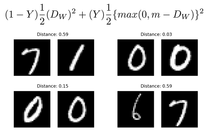
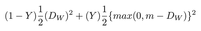
• The value is our label. It will be if the image pairs are of the same class, and it will be if the image pairs are of a different class.
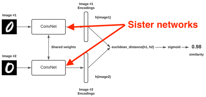
• The variable is the Euclidean distance between the outputs of the sister network embeddings.
• The max function takes the largest value of and the margin, , minus the distance.

We’ll be implementing this loss function using Keras and TensorFlow later in this tutorial.

If you would like more mathematically motivated details on contrastive loss, be sure to refer to Hadsell et al.’s paper, Dimensionality Reduction by Learning an Invariant Mapping.

Configuring your development environment

This series of tutorials on siamese networks utilizes Keras and TensorFlow. If you intend on following this tutorial on the previous two parts in this series, I suggest you take the time now to configure your deep learning development environment.

You can utilize either of these two guides to install TensorFlow and Keras on your system:

• How to install TensorFlow 2.0 on Ubuntu
• How to install TensorFlow 2.0 on macOS

Either tutorial will help you configure your system with all the necessary software for this blog post in a convenient Python virtual environment.

Having problems configuring your development environment?

All that said, are you:

• Short on time?
• Learning on your employer’s administratively locked system?
• Wanting to skip the hassle of fighting with the command line, package managers, and virtual environments?
• Ready to run the code right now on your Windows, macOS, or Linux system?

Then join PyImageSearch Plus today!

Gain access to Jupyter Notebooks for this tutorial and other PyImageSearch guides that are pre-configured to run on Google Colab’s ecosystem right in your web browser! No installation required.

And best of all, these Jupyter Notebooks will run on Windows, macOS, and Linux!

Project structure

Today’s tutorial on contrastive loss on siamese networks builds on my three previous tutorials that cover the fundamentals of building image pairs, implementing and training siamese networks, and using siamese networks for inference:

1. Building image pairs for siamese networks with Python
2. Siamese networks with Keras, TensorFlow, and Deep Learning
3. Comparing images for similarity using siamese networks, Keras, and TensorFlow

We’ll be building on the knowledge we gained from those guides (including the project directory structure itself) today, so consider the previous guides required reading before continuing today.

Once you’ve gotten caught up, we can proceed to review our project directory structure:

$ tree . --dirsfirst
.
├── examples
│   ├── image_01.png
│   ├── image_02.png
│   ├── image_03.png
...
│   └── image_13.png
├── output
│   ├── contrastive_siamese_model
│   │   ├── assets
│   │   ├── variables
│   │   │   ├── variables.data-00000-of-00001
│   │   │   └── variables.index
│   │   └── saved_model.pb
│   └── contrastive_plot.png
├── pyimagesearch
│   ├── config.py
│   ├── metrics.py
│   ├── siamese_network.py
│   └── utils.py
├── test_contrastive_siamese_network.py
└── train_contrastive_siamese_network.py

6 directories, 23 files

Again, I cannot stress the importance of reviewing my previous series of tutorials on siamese networks. Doing so is an absolute requirement before continuing here today.

Implementing our configuration file

Our configuration file holds important variables used to train our siamese network with contrastive loss.

Open up the config.py file in your project directory structure, and let’s take a look inside:

# import the necessary packages
import os

# specify the shape of the inputs for our network
IMG_SHAPE = (28, 28, 1)

# specify the batch size and number of epochs
BATCH_SIZE = 64
EPOCHS = 100

# define the path to the base output directory
BASE_OUTPUT = "output"

# use the base output path to derive the path to the serialized
# model along with training history plot
MODEL_PATH = os.path.sep.join([BASE_OUTPUT,
	"contrastive_siamese_model"])
PLOT_PATH = os.path.sep.join([BASE_OUTPUT,
	"contrastive_plot.png"])

Lines 16-19 define the output file paths for both our serialized model and training history.

For more details on the configuration file, refer to my tutorial on Siamese networks with Keras, TensorFlow, and Deep Learning.

Creating our helper utility functions

# import the necessary packages
import tensorflow.keras.backend as K
import matplotlib.pyplot as plt
import numpy as np

We then have our make_pairs function, which I discussed in detail in my Building image pairs for siamese networks with Python tutorial (make sure you read that guide before continuing):

def make_pairs(images, labels):
	# initialize two empty lists to hold the (image, image) pairs and
	# labels to indicate if a pair is positive or negative
	pairImages = []
	pairLabels = []

	# calculate the total number of classes present in the dataset
	# and then build a list of indexes for each class label that
	# provides the indexes for all examples with a given label
	numClasses = len(np.unique(labels))
	idx = [np.where(labels == i)[0] for i in range(0, numClasses)]

	# loop over all images
	for idxA in range(len(images)):
		# grab the current image and label belonging to the current
		# iteration
		currentImage = images[idxA]
		label = labels[idxA]

		# randomly pick an image that belongs to the *same* class
		# label
		idxB = np.random.choice(idx[label])
		posImage = images[idxB]

		# prepare a positive pair and update the images and labels
		# lists, respectively
		pairImages.append([currentImage, posImage])
		pairLabels.append([1])

		# grab the indices for each of the class labels *not* equal to
		# the current label and randomly pick an image corresponding
		# to a label *not* equal to the current label
		negIdx = np.where(labels != label)[0]
		negImage = images[np.random.choice(negIdx)]

		# prepare a negative pair of images and update our lists
		pairImages.append([currentImage, negImage])
		pairLabels.append([0])

	# return a 2-tuple of our image pairs and labels
	return (np.array(pairImages), np.array(pairLabels))

def euclidean_distance(vectors):
	# unpack the vectors into separate lists
	(featsA, featsB) = vectors

	# compute the sum of squared distances between the vectors
	sumSquared = K.sum(K.square(featsA - featsB), axis=1,
		keepdims=True)

	# return the euclidean distance between the vectors
	return K.sqrt(K.maximum(sumSquared, K.epsilon()))

Finally, we have a helper utility, plot_training, which accepts a plotPath, plots our training and validation contrastive loss over the course of training, and then saves the plot to disk:

def plot_training(H, plotPath):
	# construct a plot that plots and saves the training history
	plt.style.use("ggplot")
	plt.figure()
	plt.plot(H.history["loss"], label="train_loss")
	plt.plot(H.history["val_loss"], label="val_loss")
	plt.title("Training Loss")
	plt.xlabel("Epoch #")
	plt.ylabel("Loss")
	plt.legend(loc="lower left")
	plt.savefig(plotPath)

Let’s move on to implementing the siamese network architecture itself.

Implementing our siamese network architecture

Our siamese neural network architecture is essentially a basic CNN:

# import the necessary packages
from tensorflow.keras.models import Model
from tensorflow.keras.layers import Input
from tensorflow.keras.layers import Conv2D
from tensorflow.keras.layers import Dense
from tensorflow.keras.layers import Dropout
from tensorflow.keras.layers import GlobalAveragePooling2D
from tensorflow.keras.layers import MaxPooling2D

def build_siamese_model(inputShape, embeddingDim=48):
	# specify the inputs for the feature extractor network
	inputs = Input(inputShape)

	# define the first set of CONV => RELU => POOL => DROPOUT layers
	x = Conv2D(64, (2, 2), padding="same", activation="relu")(inputs)
	x = MaxPooling2D(pool_size=(2, 2))(x)
	x = Dropout(0.3)(x)

	# second set of CONV => RELU => POOL => DROPOUT layers
	x = Conv2D(64, (2, 2), padding="same", activation="relu")(x)
	x = MaxPooling2D(pool_size=2)(x)
	x = Dropout(0.3)(x)

	# prepare the final outputs
	pooledOutput = GlobalAveragePooling2D()(x)
	outputs = Dense(embeddingDim)(pooledOutput)

	# build the model
	model = Model(inputs, outputs)

	# return the model to the calling function
	return model

You can refer to my tutorial on Siamese networks with Keras, TensorFlow, and Deep Learning for more details on the model architecture and implementation.

Implementing contrastive loss with Keras and TensorFlow

The full implementation of contrastive loss is concise, spanning only 18 lines, including comments:

# import the necessary packages
import tensorflow.keras.backend as K
import tensorflow as tf

def contrastive_loss(y, preds, margin=1):
	# explicitly cast the true class label data type to the predicted
	# class label data type (otherwise we run the risk of having two
	# separate data types, causing TensorFlow to error out)
	y = tf.cast(y, preds.dtype)

	# calculate the contrastive loss between the true labels and
	# the predicted labels
	squaredPreds = K.square(preds)
	squaredMargin = K.square(K.maximum(margin - preds, 0))
	loss = K.mean(y * squaredPreds + (1 - y) * squaredMargin)

	# return the computed contrastive loss to the calling function
	return loss

I suggest you review the “What is contrastive loss? And how can contrastive loss be used to train siamese networks?” section above and compare our implementation to the equation so you can better understand how contrastive loss is implemented.

Creating our contrastive loss training script

We are now ready to implement our training script! This script is responsible for:

1. Loading the MNIST digits dataset from disk
2. Preprocessing it and constructing image pairs
3. Instantiating the siamese neural network architecture
4. Training the siamese network with contrastive loss
5. Serializing both the trained network and training history plot to disk

The majority of this code is identical to our previous post on Siamese networks with Keras, TensorFlow, and Deep Learning, so while I’m still going to cover our implementation in full, I’m going to defer a detailed discussion to the previous post (and of course, pointing out the details along the way).

Open up the train_contrastive_siamese_network.py file in your project directory structure, and let’s get to work:

# import the necessary packages
from pyimagesearch.siamese_network import build_siamese_model
from pyimagesearch import metrics
from pyimagesearch import config
from pyimagesearch import utils
from tensorflow.keras.models import Model
from tensorflow.keras.layers import Dense
from tensorflow.keras.layers import Input
from tensorflow.keras.layers import Lambda
from tensorflow.keras.datasets import mnist
import numpy as np

# load MNIST dataset and scale the pixel values to the range of [0, 1]
print("[INFO] loading MNIST dataset...")
(trainX, trainY), (testX, testY) = mnist.load_data()
trainX = trainX / 255.0
testX = testX / 255.0

# add a channel dimension to the images
trainX = np.expand_dims(trainX, axis=-1)
testX = np.expand_dims(testX, axis=-1)

# prepare the positive and negative pairs
print("[INFO] preparing positive and negative pairs...")
(pairTrain, labelTrain) = utils.make_pairs(trainX, trainY)
(pairTest, labelTest) = utils.make_pairs(testX, testY)

Line 15 loads the MNIST dataset with the pre-supplied training and testing splits.

We then preprocess the dataset by:

1. Scaling the input pixel intensities in the images from the range [0, 255] to [0, 1] (Lines 16 and 17)
2. Adding a channel dimension (Lines 20 and 21)
3. Constructing our image pairs (Lines 25 and 26)

Next, we can instantiate the siamese network architecture:

# configure the siamese network
print("[INFO] building siamese network...")
imgA = Input(shape=config.IMG_SHAPE)
imgB = Input(shape=config.IMG_SHAPE)
featureExtractor = build_siamese_model(config.IMG_SHAPE)
featsA = featureExtractor(imgA)
featsB = featureExtractor(imgB)

# finally, construct the siamese network
distance = Lambda(utils.euclidean_distance)([featsA, featsB])
model = Model(inputs=[imgA, imgB], outputs=distance)

Lines 30-34 create our sister networks:

• We start by creating two inputs, one for each image in the image pair (Lines 30 and 31).
• We then build the sister network architecture, which acts as our feature extractor (Line 32).
• Each image in the pair will be passed through our feature extractor, resulting in a vector that quantifies each image (Lines 33 and 34).

# compile the model
print("[INFO] compiling model...")
model.compile(loss=metrics.contrastive_loss, optimizer="adam")

# train the model
print("[INFO] training model...")
history = model.fit(
	[pairTrain[:, 0], pairTrain[:, 1]], labelTrain[:],
	validation_data=([pairTest[:, 0], pairTest[:, 1]], labelTest[:]),
	batch_size=config.BATCH_SIZE,
	epochs=config.EPOCHS)

# serialize the model to disk
print("[INFO] saving siamese model...")
model.save(config.MODEL_PATH)

# plot the training history
print("[INFO] plotting training history...")
utils.plot_training(history, config.PLOT_PATH)

Line 42 compiles our model architecture using the contrastive_loss function.

We then proceed to train the model using our training/validation image pairs (Lines 46-50) and then serialize the model to disk (Line 54) and plot the training history (Line 58).

Training a siamese network with contrastive loss

We are now ready to train our siamese neural network with contrastive loss using Keras and TensorFlow.

Make sure you use the “Downloads” section of this guide to download the source code, helper utilities, and contrastive loss implementation.

From there, you can execute the following command:

$ python train_contrastive_siamese_network.py
[INFO] loading MNIST dataset...
[INFO] preparing positive and negative pairs...
[INFO] building siamese network...
[INFO] compiling model...
[INFO] training model...
Epoch 1/100
1875/1875 [==============================] - 81s 43ms/step - loss: 0.2038 - val_loss: 0.1755
Epoch 2/100
1875/1875 [==============================] - 80s 43ms/step - loss: 0.1756 - val_loss: 0.1571
Epoch 3/100
1875/1875 [==============================] - 80s 43ms/step - loss: 0.1619 - val_loss: 0.1394
Epoch 4/100
1875/1875 [==============================] - 81s 43ms/step - loss: 0.1548 - val_loss: 0.1356
Epoch 5/100
1875/1875 [==============================] - 81s 43ms/step - loss: 0.1501 - val_loss: 0.1262
...
Epoch 96/100
1875/1875 [==============================] - 81s 43ms/step - loss: 0.1264 - val_loss: 0.1066
Epoch 97/100
1875/1875 [==============================] - 80s 43ms/step - loss: 0.1262 - val_loss: 0.1100
Epoch 98/100
1875/1875 [==============================] - 82s 44ms/step - loss: 0.1262 - val_loss: 0.1078
Epoch 99/100
1875/1875 [==============================] - 81s 43ms/step - loss: 0.1268 - val_loss: 0.1067
Epoch 100/100
1875/1875 [==============================] - 80s 43ms/step - loss: 0.1261 - val_loss: 0.1107
[INFO] saving siamese model...
[INFO] plotting training history...

Each epoch took ~80 seconds on my 3 GHz Intel Xeon W processor. Training would be even faster with a GPU.

Our training history can be seen in Figure 7. Notice how our validation loss is actually lower than our training loss, a phenomenon that I discuss in this tutorial.

Having our validation loss lower than our training loss implies that we can “train harder” to improve our siamese network accuracy, typically by relaxing regularization constraints, deepening the model, and using a more aggressive learning rate.

But for now, our training model is more than sufficient.

Implementing our contrastive loss test script

# import the necessary packages
from pyimagesearch import config
from pyimagesearch import utils
from tensorflow.keras.models import load_model
from imutils.paths import list_images
import matplotlib.pyplot as plt
import numpy as np
import argparse
import cv2

# construct the argument parser and parse the arguments
ap = argparse.ArgumentParser()
ap.add_argument("-i", "--input", required=True,
	help="path to input directory of testing images")
args = vars(ap.parse_args())

# grab the test dataset image paths and then randomly generate a
# total of 10 image pairs
print("[INFO] loading test dataset...")
testImagePaths = list(list_images(args["input"]))
np.random.seed(42)
pairs = np.random.choice(testImagePaths, size=(10, 2))

# load the model from disk
print("[INFO] loading siamese model...")
model = load_model(config.MODEL_PATH, compile=False)

# loop over all image pairs
for (i, (pathA, pathB)) in enumerate(pairs):
	# load both the images and convert them to grayscale
	imageA = cv2.imread(pathA, 0)
	imageB = cv2.imread(pathB, 0)

	# create a copy of both the images for visualization purpose
	origA = imageA.copy()
	origB = imageB.copy()

	# add channel a dimension to both the images
	imageA = np.expand_dims(imageA, axis=-1)
	imageB = np.expand_dims(imageB, axis=-1)

	# add a batch dimension to both images
	imageA = np.expand_dims(imageA, axis=0)
	imageB = np.expand_dims(imageB, axis=0)

	# scale the pixel values to the range of [0, 1]
	imageA = imageA / 255.0
	imageB = imageB / 255.0

	# use our siamese model to make predictions on the image pair,
	# indicating whether or not the images belong to the same class
	preds = model.predict([imageA, imageB])
	proba = preds[0][0]

1. Load the two images from disk (Lines 31 and 32)
2. Clone the images such that we can visualize/draw on them (Lines 35 and 36)
3. Add a channel dimension to both images, a requirement for inference (Lines 39 and 40)
4. Add a batch dimension to the images, again, a requirement for inference (Lines 43 and 44)
5. Scale the pixel intensities from the range [0, 255] to [0, 1], just like we did during training

The image pairs are then passed through our siamese network on Lines 52 and 53, resulting in the computed Euclidean distance between the vectors generated by the sister networks.

Again, keep in mind that the smaller the distance is, the more similar the two images are. Conversely, the larger the distance, the less similar the images are.

The final code block handles visualizing the two images in the pair along with their computed distance:

	# initialize the figure
	fig = plt.figure("Pair #{}".format(i + 1), figsize=(4, 2))
	plt.suptitle("Distance: {:.2f}".format(proba))

	# show first image
	ax = fig.add_subplot(1, 2, 1)
	plt.imshow(origA, cmap=plt.cm.gray)
	plt.axis("off")

	# show the second image
	ax = fig.add_subplot(1, 2, 2)
	plt.imshow(origB, cmap=plt.cm.gray)
	plt.axis("off")

	# show the plot
	plt.show()

Congratulations on implementing an inference script for siamese networks! For more details on this implementation, refer to my previous tutorial, Comparing images for similarity using siamese networks, Keras, and TensorFlow.

Making predictions using our siamese network with contrastive loss model

$ python test_contrastive_siamese_network.py --input examples
[INFO] loading test dataset...
[INFO] loading siamese model...

Looking at Figure 8, you’ll see that we have sets of example image pairs presented to our siamese network trained with contrastive loss.

Images that are of the same class have lower distances while images of different classes have larger classes.

You can thus set a threshold value, T, to act as a cutoff on distance. If the computed distance, D, is < T, then the image pair must belong to the same class. Otherwise, if D >= T, then the images are different classes.

Setting the threshold T should be done empirically through experimentation:

• Train the network.
• Compute distances for image pairs.
• Manually visualize the pairs and their corresponding differences.
• Find a cutoff value that maximizes correct classifications and minimizes incorrect ones.

In this case, setting T=0.16 would be an appropriate threshold, since it allows us to correctly mark all image pairs that belong to the same class, while all image pairs of different classes are treated as such.

What’s next?

If you’re interested in learning more about siamese neural networks, I strongly recommend that you start with the fundamentals of deep learning and computer vision.

You’ll find it much easier to implement these advanced neural network architectures if you have a thorough understanding of the basics.

My book Deep Learning for Computer Vision with Python blends theory with code implementation, so you’ll build a strong foundation for your computer vision, deep learning, and artificial intelligence education.

Inside this book you learn:

• Everything you need to know about the fundamentals and theory of deep learning without unnecessary mathematical jargon. You’ll be able to understand and implement the basic equations easily because they are all backed up with code walkthroughs. You definitely don’t need a degree in advanced math to understand this book.
• How to implement state-of-the-art custom neural network architectures and create your own. By the end of the book, you’ll thoroughly understand how to implement CNNs such as ResNet, SqueezeNet, etc., and you’ll be confident to create custom neural network architectures.
• How to train CNNs on your own datasets. Unlike most deep learning tutorials, in this book you’ll learn how to work with your own custom datasets. In fact. you’ll be training CNNs on your own datasets even before you finish the book.
• Object detection (Faster R-CNNs, Single Shot Detectors, and RetinaNet) and instance segmentation (Mask R-CNN). You’ll learn how to create your own custom object detectors and segmentation networks.

You’ll also find answers and proven code recipes to:

• Create and prepare your own custom image datasets for image classification, object detection, and segmentation
• Understand the algorithms behind deep learning for computer vision and their implementations by getting real-life experience from hands-on tutorials
• Maximize the accuracy of your models by taking action with my tips and best practices

This book is packed full of highly actionable content and is delivered in the same no-nonsense teaching style you expect from PyImageSearch. If you’d like to try before you buy, click here and I’ll send you the full table of contents and some sample chapters.

Wondering how far you can go with deep learning? Check out these success stories from students who decided to take a deep dive into deep learning and computer vision.

Summary

In this tutorial you learned about contrastive loss, including how it’s a better loss function than binary cross-entropy for training siamese networks.

What you need to keep in mind here is that a siamese network isn’t specifically designed for classification. Instead, it’s utilized for differentiation, meaning that it should not only be able to tell if an image pair belongs to the same class or not but whether the two images are identical/similar or not.

Contrastive loss works far better in this situation.

I recommend you experiment with both binary cross-entropy and contrastive loss when training your own siamese neural networks, but I think you’ll find that overall, contrastive loss does a much better job.

To download the source code to this post (and be notified when future tutorials are published here on PyImageSearch), simply enter your email address in the form below!

Download the Source Code and FREE 17-page Resource Guide

Enter your email address below to get a .zip of the code and a FREE 17-page Resource Guide on Computer Vision, OpenCV, and Deep Learning. Inside you'll find my hand-picked tutorials, books, courses, and libraries to help you master CV and DL!

Download the code!

Website

The post Contrastive Loss for Siamese Networks with Keras and TensorFlow appeared first on PyImageSearch.

In this tutorial you will learn how to detect low contrast images using OpenCV and scikit-image.

Whenever I teach the fundamentals of computer vision and image processing to students eager to learn, one of the first things I teach is:

“It’s far easier to write code for images captured in controlled lighting conditions than in dynamic conditions with no guarantees.”

If you are able to control the environment and, most importantly, the lighting when you capture an image, the easier it will be to write code to process the image.

With controlled lighting conditions you’re able to hard-code parameters, including:

• Amount of blurring
• Edge detection bounds
• Thresholding limits
• Etc.

Essentially, controlled conditions allow you to take advantage of your a priori knowledge of an environment and then write code that handles that specific environment rather than trying to handle every edge case or condition.

Of course, controlling your environment and lighting conditions isn’t always possible …

… so what do you do then?

Do you try to code a super complex image processing pipeline that handles every edge case?

Well … you could do that — and probably waste weeks or months doing it and still likely not capture every edge case.

Or, you can instead detect when low quality images, specifically low contrast images, are presented to your pipeline.

If a low contrast image is detected, you can throw the image out or alert the user to capture an image in better lighting conditions.

Doing so will make it far easier for you to develop image processing pipelines (and reduce your headaches along the way).

To learn how to detect low contrast images with OpenCV and scikit-image, just keep reading.

Looking for the source code to this post?

Jump Right To The Downloads Section

Detecting low contrast images with OpenCV, scikit-image, and Python

In the first part of this tutorial, we’ll discuss what low contrast images are, the problems they cause for computer vision/image processing practitioners, and how we can programmatically detect these images.

From there we’ll configure our development environment and review our project directory structure.

With our project structure reviewed, we’ll move on to coding two Python scripts:

1. One to detect low contrast in static images
2. And another to detect low contrast frames in real-time video streams

We’ll wrap up our tutorial with a discussion of our results.

What problems do low contrast images/frames create? And how can we detect them?

A low contrast image has very little difference between light and dark regions, making it hard to see where the boundary of an object begins and the background of the scene starts.

An example of a low contrast image is shown in Figure 1 (left). Here you can see a color matching/correction card on a background. Due to poor lighting conditions (i.e., not enough light), the boundaries of the card against the background are not well defined — by itself, an edge detection algorithm, such as the Canny edge detector, may struggle to detect the boundary of the card, especially if the Canny edge detector parameters are hard-coded.

Figure 1 (right) shows an example image of “normal contrast”. We have more detail in this image due to better lighting conditions. Notice that the white of the color matching card sufficiently contrasts the background — it would be far easier for an image processing pipeline to detect the edges of the color matching card (compared to the right image).

Whenever you’re tackling a computer vision or image processing problem, always start with the environment the image/frame is captured in. The more you can control and guarantee the lighting conditions, the easier a time you will have writing code to process the scene.

However, there will be times when you cannot control the lighting conditions and any parameters you hard-coded into your pipeline (ex., blur sizes, thresholding limits, Canny edge detection parameters, etc.) may result in incorrect/unusable output.

When that inevitably happens, don’t throw in the towel. And certainly don’t start going down the rabbit hole of coding up complex image processing pipelines to handle every edge case.

Instead, leverage low contrast image detection.

Using low contrast image detection, you can programmatically detect images that are not sufficient for your image processing pipeline.

In the remainder of this tutorial, you’ll learn how to detect low contrast images in both static scenes and real-time video streams.

We’ll throw out images/frames that are low contrast and not suitable for our pipeline, while keeping only the ones that we know will produce usable results.

By the end of this guide, you’ll have a good understanding of low contrast image detection, and you’ll be able to apply it to your own projects, thereby making your own pipelines easier to develop and more stable in production.

Configuring your development environment

In order to detect low contrast images, you need to have the OpenCV library as well as scikit-image installed.

Luckily, both of these are pip-installable:

$ pip install opencv-contrib-python
$ pip install scikit-image

If you need help configuring your development environment for OpenCV and scikit-image, I highly recommend that you read my pip install OpenCV guide — it will have you up and running in a matter of minutes.

Having problems configuring your development environment?

All that said, are you:

• Short on time?
• Learning on your employer’s administratively locked system?
• Wanting to skip the hassle of fighting with the command line, package managers, and virtual environments?
• Ready to run the code right now on your Windows, macOS, or Linux system?

Then join PyImageSearch Plus today!

Gain access to Jupyter Notebooks for this tutorial and other PyImageSearch guides that are pre-configured to run on Google Colab’s ecosystem right in your web browser! No installation required.

And best of all, these Jupyter Notebooks will run on Windows, macOS, and Linux!

Project structure

Before we get too far in this guide, let’s take a second to inspect our project directory structure.

Start by using the “Downloads” section of this tutorial to download the source code, example images, and sample video:

$ tree . --dirsfirst
.
├── examples
│   ├── 01.jpg
│   ├── 02.jpg
│   └── 03.jpg
├── detect_low_contrast_image.py
├── detect_low_contrast_video.py
└── example_video.mp4

1 directory, 6 files

We have two Python scripts to review today:

1. detect_low_contrast_image.py: Performs low contrast detection in static images (i.e., images inside the examples directory)
2. detect_low_contrast_video.py: Applies low contrast detection to real-time video streams (in this case, example_video.mp4)

You can of course substitute in your own images and video files/streams as you see fit.

Implementing low contrast image detection with OpenCV

Let’s learn how to detect low contrast images with OpenCV and scikit-image!

Open up the detect_low_contrast_image.py file in your project directory structure, and insert the following code.

# import the necessary packages
from skimage.exposure import is_low_contrast
from imutils.paths import list_images
import argparse
import imutils
import cv2

We start off on Lines 2-6 importing our required Python packages.

# construct the argument parser and parse the arguments
ap = argparse.ArgumentParser()
ap.add_argument("-i", "--input", required=True,
	help="path to input directory of images")
ap.add_argument("-t", "--thresh", type=float, default=0.35,
	help="threshold for low contrast")
args = vars(ap.parse_args())

We have two command line arguments, the first of which is required and the second optional:

1. --input: Path to our input image residing on disk
2. --thresh: The threshold for low contrast

I’ve set the --thresh parameter to a default of 0.35, implying that an image will be considered low contrast “when the range of brightness spans less than this fraction of its data type’s full range” (official scikit-image documentation).

Essentially, what this means is that if less than 35% of the range of brightness occupies the full range of the data type, then the image is considered low contrast.

To make this a concrete example, consider that an image in OpenCV is represented by an unsigned 8-bit integer that has a range of values [0, 255]. If the distribution of pixel intensities occupies less than 35% of this [0, 255] range, then the image is considered low contrast.

# grab the paths to the input images
imagePaths = sorted(list(list_images(args["input"])))

# loop over the image paths
for (i, imagePath) in enumerate(imagePaths):
	# load the input image from disk, resize it, and convert it to
	# grayscale
	print("[INFO] processing image {}/{}".format(i + 1,
		len(imagePaths)))
	image = cv2.imread(imagePath)
	image = imutils.resize(image, width=450)
	gray = cv2.cvtColor(image, cv2.COLOR_BGR2GRAY)

	# blur the image slightly and perform edge detection
	blurred = cv2.GaussianBlur(gray, (5, 5), 0)
	edged = cv2.Canny(blurred, 30, 150)

	# initialize the text and color to indicate that the input image
	# is *not* low contrast
	text = "Low contrast: No"
	color = (0, 255, 0)

1. Load the image from disk
2. Resize it to have a width of 450 pixels
3. Convert the image to grayscale

From there we apply blurring (to reduce high frequency noise) and then apply the Canny edge detector (Lines 30 and 31) to detect edges in the input image.

	# check to see if the image is low contrast
	if is_low_contrast(gray, fraction_threshold=args["thresh"]):
		# update the text and color
		text = "Low contrast: Yes"
		color = (0, 0, 255)

	# otherwise, the image is *not* low contrast, so we can continue
	# processing it
	else:
		# find contours in the edge map and find the largest one,
		# which we'll assume is the outline of our color correction
		# card
		cnts = cv2.findContours(edged.copy(), cv2.RETR_EXTERNAL,
			cv2.CHAIN_APPROX_SIMPLE)
		cnts = imutils.grab_contours(cnts)
		c = max(cnts, key=cv2.contourArea)

		# draw the largest contour on the image
		cv2.drawContours(image, [c], -1, (0, 255, 0), 2)

	# draw the text on the output image
	cv2.putText(image, text, (5, 25), cv2.FONT_HERSHEY_SIMPLEX, 0.8,
		color, 2)

	# show the output image and edge map
	cv2.imshow("Image", image)
	cv2.imshow("Edge", edged)
	cv2.waitKey(0)

Otherwise, the image is not low contrast, so we can proceed with our image processing pipeline (Lines 46-56). Inside this code block we:

1. Find contours in our edge map
2. Find the largest contour in our cnts list (which we assume will be our card in the input image)
3. Draw the outline of the card on the image

Finally, we draw the text on the image and display both the image and edge map to our screen.

Low contrast image detection results

Let’s now apply low contrast image detection to our own images!

Start by using the “Downloads” section of this tutorial to download the the source code and example images:

$ python detect_low_contrast_image.py --input examples
[INFO] processing image 1/3
[INFO] processing image 2/3
[INFO] processing image 3/3

Our first image here is labeled as “low contrast”. As you can see, applying the Canny edge detector to the low contrast image results in us being unable to detect the outline of the card in the image.

If we tried to process this image further and detected the card itself, we would end up detecting some other contour. Instead, by applying low contrast detection, we can simply ignore the image.

Our second image has sufficient contrast, and as such, we are able to accurately compute the edge map and extract the contour associated with the card outline:

Our final image is also labeled as having sufficient contrast:

We are again able to compute the edge map, perform contour detection, and extract the contour associated with the outline of the card.

Implementing low contrast frame detection in real-time video streams

In this section you will learn how to implement low contrast frame detection in real-time video streams using OpenCV and Python.

Open up the detect_low_contrast_video.py file in your project directory structure, and let’s get to work:

# import the necessary packages
from skimage.exposure import is_low_contrast
import numpy as np
import argparse
import imutils
import cv2

# construct the argument parser and parse the arguments
ap = argparse.ArgumentParser()
ap.add_argument("-i", "--input", type=str, default="",
	help="optional path to video file")
ap.add_argument("-t", "--thresh", type=float, default=0.35,
	help="threshold for low contrast")
args = vars(ap.parse_args())

# grab a pointer to the input video stream
print("[INFO] accessing video stream...")
vs = cv2.VideoCapture(args["input"] if args["input"] else 0)

# loop over frames from the video stream
while True:
	# read a frame from the video stream
	(grabbed, frame) = vs.read()

	# if the frame was not grabbed then we've reached the end of
	# the video stream so exit the script
	if not grabbed:
		print("[INFO] no frame read from stream - exiting")
		break

	# resize the frame, convert it to grayscale, blur it, and then
	# perform edge detection
	frame = imutils.resize(frame, width=450)
	gray = cv2.cvtColor(frame, cv2.COLOR_BGR2GRAY)
	blurred = cv2.GaussianBlur(gray, (5, 5), 0)
	edged = cv2.Canny(blurred, 30, 150)

	# initialize the text and color to indicate that the current
	# frame is *not* low contrast
	text = "Low contrast: No"
	color = (0, 255, 0)

Line 18 instantiates a point to our video stream. By default we’ll use our webcam; however, if you are a video file, you can supply the --input command line argument.

We then loop over frames from the video stream on Line 21. Inside the loop we:

1. Read the next frame
2. Detect whether we’ve reached the end of the video stream, and if so, break from the loop
3. Preprocess the frame by converting it to grayscale, blurring it, and applying the Canny edge detector

	# check to see if the frame is low contrast, and if so, update
	# the text and color
	if is_low_contrast(gray, fraction_threshold=args["thresh"]):
		text = "Low contrast: Yes"
		color = (0, 0, 255)

	# otherwise, the frame is *not* low contrast, so we can continue
	# processing it
	else:
		# find contours in the edge map and find the largest one,
		# which we'll assume is the outline of our color correction
		# card
		cnts = cv2.findContours(edged.copy(), cv2.RETR_EXTERNAL,
			cv2.CHAIN_APPROX_SIMPLE)
		cnts = imutils.grab_contours(cnts)
		c = max(cnts, key=cv2.contourArea)

		# draw the largest contour on the frame
		cv2.drawContours(frame, [c], -1, (0, 255, 0), 2)

	# draw the text on the output frame
	cv2.putText(frame, text, (5, 25), cv2.FONT_HERSHEY_SIMPLEX, 0.8,
		color, 2)

	# stack the output frame and edge map next to each other
	output = np.dstack([edged] * 3)
	output = np.hstack([frame, output])

	# show the output to our screen
	cv2.imshow("Output", output)
	key = cv2.waitKey(1) & 0xFF

	# if the `q` key was pressed, break from the loop
	if key == ord("q"):
		break

Detecting low contrast frames in real-time

We are now ready to detect low contrast images in real-time video streams!

Use the “Downloads” section of this tutorial to download the source code, example images, and sample video file.

From there, open up a terminal, and execute the following command:

$ python detect_low_contrast_video.py --input example_video.mp4
[INFO] accessing video stream...
[INFO] no frame read from stream - exiting

As our output shows, our low contrast frame detector is able to detect frames with low contrast and prevent them from proceeding down the rest of our image processing pipeline.

Conversely, images with sufficient contrast are allowed to proceed. We then apply edge detection to each of these frames, compute contours, and extract the contour/outline associated with the color correction card.

You can use low contrast detection in video streams in the same manner.

What’s next?

Now that you know how to detect low contrast images using OpenCV and scikit-image, it’ll be much easier for you to develop effective image processing pipelines. And you can go deeper into the world of computer vision and add even more advanced techniques to your arsenal.

Inside the PyImageSearch Gurus course you’ll learn:

• Automatic License/Number Plate Recognition (ANPR)
• Face recognition
• Training your own custom object detector
• Deep learning and Convolutional Neural Networks
• Content-based Image Retrieval (CBIR)
• … and much more!

PyImageSearch Gurus is different from other computer vision courses because it is:

• Highly actionable. You’ll learn concepts and code through practical application and hands-on experience. And it’s all delivered in the same easy-to-understand style you’ve already experienced in the PyImageSearch blog. No unnecessary mathematical fluff. Just actionable content.
• Comprehensive. In fact, I guarantee you won’t find a more detailed computer vision course online. You get access to the best content from my personal vault of code and years of experience. So you’ll be able to take what you learn and put it into practice immediately.
• Collaborative. The PyImageSearch Gurus is a community of like-minded developers, researchers, and students who are eager to level-up their computer vision skills and collaborate on projects – just like you. The forums are also a great place to get expert advice from me and the more experienced students.

Interested to find out more? Grab the syllabus and 10 free sample lessons here.

And be sure to check out what these Gurus students did with the knowledge they gained in the program. Soon you could be enjoying similar success!

If you’re ready to take action and level-up your computer vision skills, join us inside PyImageSearch Gurus.

Summary

In this tutorial you learned how to detect low contrast images in both static scenes and real-time video streams. We used both the OpenCV library and the scikit-image package to develop our low contrast image detector.

While simple, this method can be extremely effective when used in computer vision and image processing pipelines.

One of the easiest ways to use this method is to provide feedback to your user. If a user provides your application with a low contrast image, alert them and request that they provide a higher-quality image.

Taking this approach allows you to place “guarantees” on the environment used to capture images that are ultimately presented to your pipeline. Furthermore, it helps the user understand that your application can only be used in certain scenarios and it’s on them to ensure they conform to your standards.

The gist here is to not overcomplicate your image processing pipelines. It’s far easier to write OpenCV code when you can place guarantees on the lighting conditions and environment — try to enforce these standards any way you can.

To download the source code to this post (and be notified when future tutorials are published here on PyImageSearch), simply enter your email address in the form below!

Download the Source Code and FREE 17-page Resource Guide

Enter your email address below to get a .zip of the code and a FREE 17-page Resource Guide on Computer Vision, OpenCV, and Deep Learning. Inside you'll find my hand-picked tutorials, books, courses, and libraries to help you master CV and DL!

Download the code!

Website

The post Detecting low contrast images with OpenCV, scikit-image, and Python appeared first on PyImageSearch.

In this tutorial, you will learn how to crop images using OpenCV.

As the name suggests, cropping is the act of selecting and extracting the Region of Interest (or simply, ROI) and is the part of the image in which we are interested.

For instance, in a face detection application, we may want to crop the face from an image. And if we were developing a Python script to recognize dogs in images, we may want to crop the dog from the image once we have found it.

We already utilized cropping in our tutorial, Getting and setting pixels with OpenCV, but we’ll review it again for more completeness.

To learn how to crop images with OpenCV, just keep reading.

Looking for the source code to this post?

Jump Right To The Downloads Section

Crop Image with OpenCV

In the first part of this tutorial, we’ll discuss how we represent OpenCV images as NumPy arrays. Since each image is a NumPy array, we can leverage NumPy array slicing to crop an image.

From there, we’ll configure our development environments and review our project directory structure.

I’ll then demonstrate how simple it is to crop images with OpenCV!

Understanding image cropping with OpenCV and NumPy array slicing

When we crop an image, we want to remove the outer parts of the image we are not interested in. We commonly refer to this process as selecting our Region of Interest, or more simply, our ROI.

We can accomplish image cropping by using NumPy array slicing.

Let’s start by initializing a NumPy list with values ranging from [0, 24]:

>>> import numpy as np
>>> I = np.arange(0, 25)
>>> I
array([ 0,  1,  2,  3,  4,  5,  6,  7,  8,  9, 10, 11, 12, 13, 14,
       15, 16, 17, 18, 19, 20, 21, 22, 23, 24])
>>> 

And let’s now reshape this 1D list into a 2D matrix, pretending that it is an image:

>>> I = I.reshape((5, 5))
>>> I
array([[ 0,  1,  2,  3,  4],
       [ 5,  6,  7,  8,  9],
       [10, 11, 12, 13, 14],
       [15, 16, 17, 18, 19],
       [20, 21, 22, 23, 24]])
>>> 

Now, let’s suppose I want to extract the “pixels” starting at x = 0, y = 0 and ending at x = 2, y = 3. Doing so can be accomplished using the following code:

>>> I[0:3, 0:2]
array([[ 0,  1],
       [ 5,  6],
       [10, 11]])
>>> 

Notice how we have extracted three rows (y = 3) and two columns (x = 2).

Now, let’s extract the pixels starting at x = 1, y = 3 and ending at x = 5 and y = 5:

>>> I[3:5, 1:5]
array([[16, 17, 18, 19],
       [21, 22, 23, 24]])
>>>

This result provides the final two rows of the image, minus the first column.

Are you noticing a pattern here?

When applying NumPy array slicing to images, we extract the ROI using the following syntax:

roi = image[startY:endY, startX:endX]

The startY:endY slice provides our rows (since the y-axis is our number of rows) while startX:endX provides our columns (since the x-axis is the number of columns) in the image. Take a second now to convince yourself that the above statement is true.

But if you’re a bit more confused and need more convincing, don’t worry! I’ll show you some code examples later in this guide to make image cropping with OpenCV more clear and concrete for you.

Configuring your development environment

To follow this guide, you need to have the OpenCV library installed on your system.

Luckily, OpenCV is pip-installable:

$ pip install opencv-contrib-python

If you need help configuring your development environment for OpenCV, I highly recommend that you read my pip install OpenCV guide — it will have you up and running in a matter of minutes.

Having problems configuring your development environment?

All that said, are you:

• Short on time?
• Learning on your employer’s administratively locked system?
• Wanting to skip the hassle of fighting with the command line, package managers, and virtual environments?
• Ready to run the code right now on your Windows, macOS, or Linux system?

Then join PyImageSearch Plus today!

Gain access to Jupyter Notebooks for this tutorial and other PyImageSearch guides that are pre-configured to run on Google Colab’s ecosystem right in your web browser! No installation required.

And best of all, these Jupyter Notebooks will run on Windows, macOS, and Linux!

Project structure

Before we can implement image cropping with OpenCV, let’s first review our project directory structure.

Start by using the “Downloads” section of this guide to access the source code and example images:

$ tree . --dirsfirst
.
├── adrian.png
└── opencv_crop.py

0 directories, 2 files

We only have a single Python script to review today, opencv_crop.py, which will load the input adrian.png image from disk and then crop out the face and body from the image using NumPy array slicing.

Implementing image cropping with OpenCV

We are now ready to implement image cropping with OpenCV.

Open the opencv_crop.py file in your project directory structure and insert the following code:

# import the necessary packages
import argparse
import cv2

# construct the argument parser and parse the arguments
ap = argparse.ArgumentParser()
ap.add_argument("-i", "--image", type=str, default="adrian.png",
	help="path to the input image")
args = vars(ap.parse_args())

Lines 2 and 3 import our required Python packages while Lines 6-9 parse our command line arguments.

We only need one command line argument, --image, which is the path to the input image we wish to crop. For this example, we’ll default the --image switch to the adrian.png file in our project directory.

Next, let’s load our image from disk:

# load the input image and display it to our screen
image = cv2.imread(args["image"])
cv2.imshow("Original", image)

# cropping an image with OpenCV is accomplished via simple NumPy
# array slices in startY:endY, startX:endX order -- here we are
# cropping the face from the image (these coordinates were
# determined using photo editing software such as Photoshop,
# GIMP, Paint, etc.)
face = image[85:250, 85:220]
cv2.imshow("Face", face)
cv2.waitKey(0)

Lines 12 and 13 load our original image and then display it to our screen:

Our goal here is to extract my face and body from the region using simple cropping methods.

We would normally apply object detection techniques to detect my face and body in the image. However, since we are still relatively early in our OpenCV education course, we will use our a priori knowledge of the image and manually supply the NumPy array slices where the body and face reside.

Again, we can, of course, use object detection methods to detect and extract faces from images automatically, but for the time being, let’s keep things simple.

We extract my face from the image on a single line of code (Line 20).

We are supplying NumPy array slices to extract a rectangular region of the image, starting at (85, 85) and ending at (220, 250).

The order in which we supply the indexes to the crop may seem counterintuitive; however, remember that OpenCV represents images as NumPy arrays with the height first (# of rows) and the width second (# of columns).

To perform our cropping, NumPy expects four indexes:

• Start y: The starting y-coordinate. In this case, we start at y = 85.
• End y: The ending y-coordinate. We will end our crop at y = 250.
• Start x: The starting x-coordinate of the slice. We start the crop at x = 85.
• End x: The ending x-axis coordinate of the slice. Our slice ends at x = 220.

We can see the result of cropping my face below:

Similarly, we can crop my body from the image:

# apply another image crop, this time extracting the body
body = image[90:450, 0:290]
cv2.imshow("Body", body)
cv2.waitKey(0)

Cropping my body is accomplished by starting the crop from coordinates (0, 90) and ending at (290, 450) of the original image.

Below you can see the output of cropping with OpenCV:

While simple, cropping is an extremely important skill that we will utilize throughout this series. If you are still feeling uneasy with cropping, definitely take the time to practice now and hone your skills. From here on, cropping will be an assumed skill that you will need to understand!

OpenCV image cropping results

To crop images with OpenCV, be sure you have gone to the “Downloads” section of this tutorial to access the source code and example images.

From there, open a shell and execute the following command:

$ python opencv_crop.py

Your cropping output should match mine from the previous section.

What’s next?

Would you like to learn how to successfully and confidently apply OpenCV to your projects?

Are you worried that configuring your development environment for Computer Vision, Deep Learning, and OpenCV will be too challenging, resulting in confusing, hard to debug error messages?

Concerned that you’ll get lost sifting through endless tutorials and video guides on your own as you struggle to master Computer Vision?

Great, because I’ve got you covered. PyImageSearch University is your chance to learn from me at your own pace.

You’ll find everything you need to master the basics (like we did together in this tutorial) and move on to advanced concepts.

Don’t worry about your operating system or development environment. I’ve got you covered with pre-configured Jupyter Notebooks in Google Colab for every tutorial on PyImageSearch, including Jupyter Notebooks for our new weekly tutorials as well!

Best of all, these Jupyter Notebooks will run on your machine, regardless of whether you are using Windows, macOS, or Linux! Irrespective of the operating system used, you will still be able to follow along and run the code in every lesson (all inside the convenience of your web browser).

Additionally, you can massively accelerate your progress by watching our video lessons accompanying each post. Every lesson in PyImageSearch University includes a detailed, step-by-step video guide.

You may feel that learning Computer Vision, Deep Learning, and OpenCV is too hard. Don’t worry; I’ll guide you gradually through each lecture and topic, so we build a solid foundation, and you grasp all the content.

When you think about it, PyImageSearch University is almost an unfair advantage compared to self-guided learning. You’ll learn more efficiently and master Computer Vision faster.

Oh, and did I mention you’ll also receive Certificates of Completion as you progress through each course at PyImageSearch University?

I’m sure PyImageSearch University will help you master OpenCV drawing and all the other computer vision skills you will need. Why not join today?

Summary

In this tutorial, you learned how to crop an image using OpenCV. Since OpenCV represents images as NumPy arrays, cropping is as simple as supplying the crop’s starting and ending ranges as a NumPy array slice.

All you need to do is remember the following syntax:

cropped = image[startY:endY, startX:endX]

As long as you remember the order in which to supply the starting and ending (x, y)-coordinates, cropping images with OpenCV is a breeze!

To download the source code to this post (and be notified when future tutorials are published here on PyImageSearch), simply enter your email address in the form below!

Download the Source Code and FREE 17-page Resource Guide

Enter your email address below to get a .zip of the code and a FREE 17-page Resource Guide on Computer Vision, OpenCV, and Deep Learning. Inside you'll find my hand-picked tutorials, books, courses, and libraries to help you master CV and DL!

Download the code!

Website

The post Crop Image with OpenCV appeared first on PyImageSearch.

In this tutorial, you will learn how to perform image arithmetic (addition and subtraction) with OpenCV.

Remember way, way back when you studied how to add and subtract numbers in grade school?

Well, it turns out, performing arithmetic with images is quite similar — with only a few caveats, of course.

In this blog post, you’ll learn how to add and subtract images, along with two important differences you need to understand regarding arithmetic operations in OpenCV and Python.

To learn how to perform image arithmetic with OpenCV, just keep reading.

Looking for the source code to this post?

Jump Right To The Downloads Section

Image Arithmetic OpenCV

In the first part of this guide, we’ll discuss what image arithmetic is, including where you see image arithmetic in real-world applications.

From there, we’ll configure our development environment and review our project directory structure.

I’ll then show you two ways to perform image arithmetic:

1. The first way is to use OpenCV’s cv2.add and cv2.subtract
2. The second way is to use NumPy’s basic addition and subtraction operators

There are very important caveats you need to understand between the two, so be sure you pay attention as you review this tutorial!

What is image arithmetic?

Image arithmetic is simply matrix addition (with an added caveat on data types, which we’ll explain later).

Let’s take a second and review some very basic linear algebra. Suppose we were to add the following two matrices:

What would the output of the matrix addition be?

The answer is simply the element-wise sum of matrix entries:

Pretty simple, right?

So it’s obvious at this point that we all know basic arithmetic operations like addition and subtraction. But when working with images, we need to keep in mind the numerical limits of our color space and data type.

For example, RGB images have pixels that fall within the range [0, 255]. What happens if we examine a pixel with an intensity of 250 and try to add 10 to it?

Under normal arithmetic rules, we would end up with a value of 260. However, since we represent RGB images as 8-bit unsigned integers who can only take on values in the range [0, 255], 260 is not a valid value.

So what should happen? Should we perform a check of some sort to ensure no pixel falls outside the range of [0, 255], thus clipping all pixels to have a minimum value of 0 and a maximum value of 255?

Or do we apply a modulus operation and “wrap around” (which is what NumPy does)? Under modulus rules, adding 10 to 255 would simply wrap around to a value of 9.

Which way is the “correct” way to handle image additions and subtractions that fall outside the range of [0, 255]?

The answer is that there is no “correct way” — it simply depends on how you are manipulating your pixels and what you want the desired results to be.

However, be sure to keep in mind that there is a difference between OpenCV and NumPy addition. NumPy will perform modulus arithmetic and “wrap around.” On the other hand, OpenCV will perform clipping and ensure pixel values never fall outside the range [0, 255].

But don’t worry! These nuances will become more clear as we explore some code below.

What is image arithmetic used for?

Now that we understand the basics of image arithmetic, you may be wondering where we would use image arithmetic in the real world.

Basic examples include:

• Adjusting brightness and contrast by adding or subtracting a set amount (for example, adding 50 to all pixel values to increase the brightness of an image)
• Working with alpha blending and transparency, as we do in this tutorial
• Creating Instagram-like filters — these filters are simply mathematical functions applied to the pixel intensities

While you may be tempted to quickly gloss over this guide on image arithmetic and move on to more advanced topics, I strongly encourage you to read this tutorial in detail. While simplistic, image arithmetic is used in many computer vision and image processing applications (whether you realize it or not).

Configuring your development environment

To follow this guide, you need to have the OpenCV library installed on your system.

Luckily, OpenCV is pip-installable:

$ pip install opencv-contrib-python

If you need help configuring your development environment for OpenCV, I highly recommend that you read my pip install OpenCV guide — it will have you up and running in a matter of minutes.

Having problems configuring your development environment?

All that said, are you:

• Short on time?
• Learning on your employer’s administratively locked system?
• Wanting to skip the hassle of fighting with the command line, package managers, and virtual environments?
• Ready to run the code right now on your Windows, macOS, or Linux system?

Then join PyImageSearch Plus today!

Gain access to Jupyter Notebooks for this tutorial and other PyImageSearch guides that are pre-configured to run on Google Colab’s ecosystem right in your web browser! No installation required.

And best of all, these Jupyter Notebooks will run on Windows, macOS, and Linux!

Project structure

Ready to learn the fundamentals of image arithmetic with OpenCV?

Great, let’s get going.

Start by using the “Downloads” section of this tutorial to access the source code and example images:

$ tree . --dirsfirst
.
├── grand_canyon.png
└── image_arithmetic.py

0 directories, 2 files

Our image_arithmetic.py file will demonstrate the differences/caveats between addition and subtraction operations in OpenCV versus NumPy.

You’ll then learn how to manually adjust the brightness of an image, grand_canyon.png, using image arithmetic with OpenCV.

Implementing image arithmetic with OpenCV

We are now ready to explore image arithmetic with OpenCV and NumPy.

Open the image_arithmetic.py file in your project folder, and let’s get started:

# import the necessary packages
import numpy as np
import argparse
import cv2

# construct the argument parser and parse the arguments
ap = argparse.ArgumentParser()
ap.add_argument("-i", "--image", type=str, default="grand_canyon.png",
	help="path to the input image")
args = vars(ap.parse_args())

Lines 2-4 import our required Python packages. Notice how we are importing NumPy for numerical array processing.

Lines 7-10 then parse our command line arguments. We need only a single switch here, --image, which points to the image on disk where we’ll be applying image arithmetic operations. We’ll default the image path to the grand_canyon.png image on disk, but you can easily update the switch if you wish to use your own image(s).

Remember how I mentioned the difference between OpenCV and NumPy arithmetic above? Well, now we are going to explore it further and provide a concrete example to ensure we fully understand it:

# images are NumPy arrays stored as unsigned 8-bit integers (unit8)
# with values in the range [0, 255]; when using the add/subtract
# functions in OpenCV, these values will be *clipped* to this range,
# even if they fall outside the range [0, 255] after applying the
# operation
added = cv2.add(np.uint8([200]), np.uint8([100]))
subtracted = cv2.subtract(np.uint8([50]), np.uint8([100]))
print("max of 255: {}".format(added))
print("min of 0: {}".format(subtracted))

On Line 17, we define two NumPy arrays that are 8-bit unsigned integers. The first array has one element: a value of 200. The second array has only one element but a value of 100. We then use OpenCV’s cv2.add method to add the values together.

What do you think the output is going to be?

According to standard arithmetic rules, we would think the result should be 300, but remember that we are working with 8-bit unsigned integers that only have a range between [0, 255].

Since we are using the cv2.add method, OpenCV takes care of clipping for us and ensures that the addition produces a maximum value of 255.

When we execute this code, we can see the result on the first line in the listing below:

max of 255: [[255]]

Sure enough, the addition returned a value of 255.

Line 20 then performs subtraction using cv2.subtract. Again, we define two NumPy arrays, each with a single element, and of the 8-bit unsigned integer data type. The first array has a value of 50 and the second a value of 100.

According to our arithmetic rules, the subtraction should return a value of -50; however, OpenCV once again performs clipping for us. We find that the value is clipped to a value of 0. Our output below verifies this:

min of 0: [[0]]

Subtracting 100 from 50 using cv2.subtract returns a value of 0.

But what happens if we use NumPy to perform the arithmetic instead of OpenCV?

Let’s explore that now:

# using NumPy arithmetic operations (rather than OpenCV operations)
# will result in a modulo ("wrap around") instead of being clipped
# to the range [0, 255]
added = np.uint8([200]) + np.uint8([100])
subtracted = np.uint8([50]) - np.uint8([100])
print("wrap around: {}".format(added))
print("wrap around: {}".format(subtracted))

First, we define two NumPy arrays, each with a single element, and of the 8-bit unsigned integer data type. The first array has a value of 200, and the second has a value of 100.

If we use the cv2.add function, our addition would be clipped and a value of 255 returned; however, NumPy does not perform clipping — it instead performs modulo arithmetic and “wraps around.”

Once a value of 255 is reached, NumPy wraps around to zero and then starts counting up again until 100 steps have been reached. You can see this is true via the first line of output below:

wrap around: [44]

Line 26 defines two more NumPy arrays: one has a value of 50 and the other 100.

When using the cv2.subtract method, this subtraction would be clipped to return a value of 0; however, we know that NumPy performs modulo arithmetic rather than clipping. Instead, once 0 is reached during the subtraction, the modulo operation wraps around and starts counting backward from 255 — we can verify this from the output below:

wrap around: [206]

It is important to keep your desired output in mind when performing integer arithmetic:

• Do you want all values to be clipped if they fall outside the range [0, 255]? Then use OpenCV’s built-in methods for image arithmetic.
• Do you want modulus arithmetic operations and have values wrap around if they fall outside the range of [0, 255]? Then simply add and subtract the NumPy arrays as you usually would.

Now that we have explored the caveats of image arithmetic in OpenCV and NumPy, let’s perform the arithmetic on actual images and view the results:

# load the original input image and display it to our screen
image = cv2.imread(args["image"])
cv2.imshow("Original", image)

We start on Lines 31 and 32 by loading our original input image from disk and then displaying it to our screen:

With our image loaded from disk, let’s proceed to increasing the brightness:

# increasing the pixel intensities in our input image by 100 is
# accomplished by constructing a NumPy array that has the *same
# dimensions* as our input image, filling it with ones, multiplying
# it by 100, and then adding the input image and matrix together
M = np.ones(image.shape, dtype="uint8") * 100
added = cv2.add(image, M)
cv2.imshow("Lighter", added)

Line 38 defines a NumPy array of ones, with the same dimensions as our image. Again, we are sure to use 8-bit unsigned integers as our data type.

To fill our matrix with values of 100s rather than 1s, we simply multiply our matrix of 1s by 100.

Finally, we use the cv2.add function to add our matrix of 100s to the original image, thus increasing every pixel intensity in the image by 100, but ensuring all values are clipped to the range [0, 255] if they attempt to exceed 255.

The result of our operation can be seen below:

Notice how the image looks more “washed out” and is substantially brighter than the original. This is because we increase the pixel intensities by adding 100 to them and pushing them toward brighter colors.

Let’s now darken our image by using cv2.subtract:

# similarly, we can subtract 50 from all pixels in our image and make it
# darker
M = np.ones(image.shape, dtype="uint8") * 50
subtracted = cv2.subtract(image, M)
cv2.imshow("Darker", subtracted)
cv2.waitKey(0)

Line 44 creates another NumPy array filled with 50s and then uses cv2.subtract to subtract 50 from each pixel in the image.

Figure 5 shows the results of this subtraction:

Our image now looks considerably darker than the original photo of the Grand Canyon. Pixels that were once white now look gray. This is because we subtract 50 from the pixels and push them toward the darker regions of the RGB color space.

OpenCV image arithmetic results

To perform image arithmetic with OpenCV and NumPy, be sure you have gone to the “Downloads” section of this tutorial to access the source code and example images.

From there, open a shell and execute the following command:

$ python image_arithmetic.py 
max of 255: [[255]]
min of 0: [[0]]
wrap around: [44]
wrap around: [206]

Your cropping output should match mine from the previous section.

What’s next?

Would you enjoy learning how to successfully and confidently apply OpenCV to your projects?

Are you worried that configuring your development environment for Computer Vision, Deep Learning, and OpenCV will be too challenging, resulting in confusing, hard to debug error messages?

Concerned that you’ll get lost sifting through endless tutorials and video guides on your own as you struggle to master Computer Vision?

Great, because I’ve got you covered. PyImageSearch University is your chance to learn from me at your own pace.

You’ll find everything you need to master the basics (like we did together in this tutorial) and move on to advanced concepts.

Don’t worry about your operating system or development environment. I’ve got you covered with pre-configured Jupyter Notebooks in Google Colab for every tutorial on PyImageSearch, including Jupyter Notebooks for our new weekly tutorials as well!

Best of all, these Jupyter Notebooks will run on your machine, regardless of whether you are using Windows, macOS, or Linux! Irrespective of the operating system used, you will still be able to follow along and run the code in every lesson (all inside the convenience of your web browser).

Additionally, you can massively accelerate your progress by watching our video lessons accompanying each post. Every lesson at PyImageSearch University includes a detailed, step-by-step video guide.

You may feel that learning Computer Vision, Deep Learning, and OpenCV is too hard. Don’t worry; I’ll guide you gradually through each lecture and topic, so we build a solid foundation, and you grasp all the content.

When you think about it, PyImageSearch University is almost an unfair advantage compared to self-guided learning. You’ll learn more efficiently and master Computer Vision faster.

Oh, and did I mention you’ll also receive Certificates of Completion as you progress through each course at PyImageSearch University?

I’m sure PyImageSearch University will help you master OpenCV drawing and all the other computer vision skills you will need. Why not join today?

Summary

In this tutorial, we learned how to apply image addition and subtraction with OpenCV, two basic (but important) image arithmetic operations.

As we saw, image arithmetic operations are simply no more than basic matrix addition and subtraction.

We also explored the peculiarities of image arithmetic using OpenCV and NumPy. Remember that:

• OpenCV addition and subtraction clip values outside the range [0, 255] to fit inside the unsigned 8-bit integer range…
• …whereas NumPy performs a modulus operation and “wraps around”

These caveats are important to keep in mind. Otherwise, you may get unwanted results when performing arithmetic operations on your images.

To download the source code to this post (and be notified when future tutorials are published here on PyImageSearch), simply enter your email address in the form below!

Download the Source Code and FREE 17-page Resource Guide

Enter your email address below to get a .zip of the code and a FREE 17-page Resource Guide on Computer Vision, OpenCV, and Deep Learning. Inside you'll find my hand-picked tutorials, books, courses, and libraries to help you master CV and DL!

Download the code!

Website

The post Image Arithmetic OpenCV appeared first on PyImageSearch.

In this tutorial, you will learn how to mask images using OpenCV.

My previous guide discussed bitwise operations, a very common set of techniques used heavily in image processing.

And as I hinted previously, we can use both bitwise operations and masks to construct ROIs that are non-rectangular. This allows us to extract regions from images that are of completely arbitrary shape.

Put simply; a mask allows us to focus only on the portions of the image that interests us.

For example, let’s say that we were building a computer vision system to recognize faces. The only part of the image we are interested in finding and describing is the parts of the image that contain faces — we simply don’t care about the rest of the image’s content. Provided that we could find the faces in the image, we may construct a mask to show only the faces in the image.

Another image masking application you’ll encounter is alpha blending and transparency (e.g., in this guide on Creating GIFs with OpenCV). When applying transparency to images with OpenCV, we need to tell OpenCV what parts of the image transparency should be applied to versus not — masks allow us to make that distinction.

To learn how to perform image masking with OpenCV, just keep reading.

Looking for the source code to this post?

Jump Right To The Downloads Section

Image Masking with OpenCV

In the first part of this tutorial, we’ll configure our development environment and review our project structure.

We’ll then implement a Python script to mask images with OpenCV.

Configuring your development environment

To follow this guide, you need to have the OpenCV library installed on your system.

Luckily, OpenCV is pip-installable:

$ pip install opencv-contrib-python

If you need help configuring your development environment for OpenCV, I highly recommend that you read my pip install OpenCV guide — it will have you up and running in a matter of minutes.

Having problems configuring your development environment?

All that said, are you:

• Short on time?
• Learning on your employer’s administratively locked system?
• Wanting to skip the hassle of fighting with the command line, package managers, and virtual environments?
• Ready to run the code right now on your Windows, macOS, or Linux systems?

Then join PyImageSearch Plus today!

Gain access to Jupyter Notebooks for this tutorial and other PyImageSearch guides that are pre-configured to run on Google Colab’s ecosystem right in your web browser! No installation required.

And best of all, these Jupyter Notebooks will run on Windows, macOS, and Linux!

Project structure

Performing image masking with OpenCV is easier than you think. But before we write any code, let’s first review our project directory structure.

Start by using the “Downloads” section of this guide to access the source code and example image.

Your project folder should look like the following:

$ tree . --dirsfirst
.
├── adrian.png
└── opencv_masking.py

0 directories, 2 files

Our opencv_masking.py script will load the input adrian.png image from disk. We’ll then use masking to extract both the body and face from the image using rectangular and circular masks, respectively.

Implementing image masking with OpenCV

Let’s learn how to apply image masking using OpenCV!

Open the opencv_masking.py file in your project directory structure, and let’s get to work:

# import the necessary packages
import numpy as np
import argparse
import cv2

# construct the argument parser and parse the arguments
ap = argparse.ArgumentParser()
ap.add_argument("-i", "--image", type=str, default="adrian.png",
	help="path to the input image")
args = vars(ap.parse_args())

Lines 2-4 import our required Python packages. We then parse our command line arguments on Lines 7-10.

We only need a single switch here, --image, which is the path to the image we want to mask. We go ahead and default the --image argument to the adrian.png file in our project directory.

Let’s now load this image from disk and perform masking:

# load the original input image and display it to our screen
image = cv2.imread(args["image"])
cv2.imshow("Original", image)

# a mask is the same size as our image, but has only two pixel
# values, 0 and 255 -- pixels with a value of 0 (background) are
# ignored in the original image while mask pixels with a value of
# 255 (foreground) are allowed to be kept
mask = np.zeros(image.shape[:2], dtype="uint8")
cv2.rectangle(mask, (0, 90), (290, 450), 255, -1)
cv2.imshow("Rectangular Mask", mask)

# apply our mask -- notice how only the person in the image is
# cropped out
masked = cv2.bitwise_and(image, image, mask=mask)
cv2.imshow("Mask Applied to Image", masked)
cv2.waitKey(0)

Lines 13 and 14 load the original image from disk and display it to our screen:

We then construct a NumPy array, filled with zeros, with the same width and height as our original image on Line 20.

As I mentioned in our previous tutorial on Image cropping with OpenCV, we can use object detection methods to detect objects/people in images automatically. Still, we’ll be using our a priori knowledge of our example image for the time being.

We know that the region we want to extract is in the image’s bottom-left corner. Line 21 draws a white rectangle on our mask, which corresponds to the region we want to extract from our original image.

Remember reviewing the cv2.bitwise_and function in our bitwise operations tutorial? It turns out that this function is used extensively when applying masks to images.

We apply our mask on Line 26 using the cv2.bitwise_and function.

The first two parameters are the image itself (i.e., the image where we want to apply the bitwise operation).

However, the important part of this function is the mask keyword. When supplied, the bitwise_and function is True when the pixel values of the input images are equal, and the mask is non-zero at each (x, y)-coordinate (in this case, only pixels that are part of the white rectangle).

After applying our mask, we display the output on Lines 27 and 28, which you can see in Figure 3:

Using our rectangular mask, we could extract only the region of the image that contains the person and ignore the rest.

Let’s look at another example, but this time using a non-rectangular mask:

# now, let's make a circular mask with a radius of 100 pixels and
# apply the mask again
mask = np.zeros(image.shape[:2], dtype="uint8")
cv2.circle(mask, (145, 200), 100, 255, -1)
masked = cv2.bitwise_and(image, image, mask=mask)

# show the output images
cv2.imshow("Circular Mask", mask)
cv2.imshow("Mask Applied to Image", masked)
cv2.waitKey(0)

On Line 32, we re-initialize our mask to be filled with zeros and the same dimensions as our original image.

Then, we draw a white circle on our mask image, starting at the center of my face with a radius of 100 pixels.

Applying the circular mask is then performed on Line 34, again using the cv2.bitwise_and function.

The results of our circular mask can be seen in Figure 4:

Here, we can see that our circle mask is shown on the left and the application of the mask on the right. Unlike the output from Figure 3, when we extracted a rectangular region, this time, we have extracted a circular region that corresponds to only my face in the image.

Furthermore, we can use this approach to extract regions from an image of arbitrary shape (rectangles, circles, lines, polygons, etc.).

OpenCV image masking results

To perform image masking with OpenCV, be sure to access the “Downloads” section of this tutorial to retrieve the source code and example image.

From there, open a shell and execute the following command:

$ python opencv_masking.py

Your masking output should match mine from the previous section.

What’s next?

Would you enjoy learning how to successfully and confidently apply OpenCV to your projects?

Are you worried that configuring your development environment for Computer Vision, Deep Learning, and OpenCV will be too challenging, resulting in confusing, hard to debug error messages?

Concerned that you’ll get lost sifting through endless tutorials and video guides on your own as you struggle to master Computer Vision?

Great, because I’ve got you covered. PyImageSearch University is your chance to learn from me at your own pace.

You’ll find everything you need to master the basics (like we did together today) and move on to advanced concepts.

Don’t worry about your operating system or development environment. I’ve got you covered with pre-configured Jupyter Notebooks in Google Colab for every tutorial on PyImageSearch, including Jupyter Notebooks for our brand new weekly tutorials as well!

Best of all, these Jupyter Notebooks will run on your machine, regardless of whether you are using Windows, macOS, or Linux! Irrespective of the operating system used, you will still be able to follow along and run the code in every lesson (all inside the convenience of your web browser).

Additionally, you can massively accelerate your progress by watching our video lessons accompanying each post. Every lesson at PyImageSearch University includes a detailed, step-by-step video guide.

You may feel like learning Computer Vision, Deep Learning, and OpenCV is too hard. Don’t worry; I’ll guide you gradually through each lecture and topic, so we build a solid foundation, and you grasp all the content.

When you think about it, PyImageSearch University is almost an unfair advantage compared to self-guided learning. You’ll learn more efficiently and master Computer Vision faster.

Oh, and did I mention you’ll also get Certificates of Completion as you progress through each course at PyImageSearch University?

I’m sure PyImageSearch University will help you master OpenCV drawing and all the other computer vision skills you will need. Why not join today?

Summary

In this tutorial, you learned the basics of masking using OpenCV.

The key point of masks is that they allow us to focus our computation only on regions of the image that interest us. Focusing our computations on regions that interest us dramatically impacts when we explore topics such as machine learning, image classification, and object detection.

For example, let’s assume that we wanted to build a system to classify the species of the flower.

In reality, we are probably only interested in the flower petals’ color and texture to perform the classification. But since we are capturing the photo in a natural environment, we’ll also have many other regions in our image, including dirt from the ground, insects, and other flowers crowding the view. How will we quantify and classify just the flower we are interested in? As we’ll see, the answer is masks.

To download the source code to this post (and be notified when future tutorials are published here on PyImageSearch), simply enter your email address in the form below!

Download the Source Code and FREE 17-page Resource Guide

Enter your email address below to get a .zip of the code and a FREE 17-page Resource Guide on Computer Vision, OpenCV, and Deep Learning. Inside you'll find my hand-picked tutorials, books, courses, and libraries to help you master CV and DL!

Download the code!

Website

The post Image Masking with OpenCV appeared first on PyImageSearch.

In this tutorial, you will learn how to apply bitwise AND, OR, XOR, and NOT with OpenCV.

In our previous tutorial on Cropping with OpenCV, you learned how to crop and extract a Region of Interest (ROI) from an image.

In that particular example, our ROI had to be rectangular . . . but what if you wanted to crop a non-rectangular region?

What would you do then?

The answer is to apply both bitwise operations and masking (we’ll discuss how to do that in our guide on image masking with OpenCV).

For now, we’ll cover the basic bitwise operations — and in the next blog post, we’ll learn how to utilize these bitwise operations to construct masks.

To learn how to apply bitwise operators with OpenCV, just keep reading.

Looking for the source code to this post?

Jump Right To The Downloads Section

OpenCV Bitwise AND, OR, XOR, and NOT

Before we get too far into this tutorial, I’m going to assume that you understand the four basic bitwise operators:

1. AND
2. OR
3. XOR (exclusive OR)
4. NOT

If you’ve never worked with bitwise operators before, I suggest you read this excellent (and highly detailed) guide from RealPython.

While you don’t have to review that guide, I find that readers who understand the basics of applying bitwise operators to digits can quickly grasp bitwise operators applied to images.

Regardless, computer vision and image processing are highly visual, and I’ve crafted the examples in this tutorial to ensure you understand how bitwise operators are applied to images with OpenCV.

We’ll start this guide by configuring our development environment and then reviewing our project directory structure.

From there, we’ll implement a Python script to perform the AND, OR, XOR, and NOT bitwise operators with OpenCV.

We’ll conclude this guide with a discussion of our results.

Configuring your development environment

To follow this guide, you need to have the OpenCV library installed on your system.

Luckily, OpenCV is pip-installable:

$ pip install opencv-contrib-python

If you need help configuring your development environment for OpenCV, I highly recommend that you read my pip install OpenCV guide — it will have you up and running in a matter of minutes.

Having problems configuring your development environment?

All that said, are you:

• Short on time?
• Learning on your employer’s administratively locked system?
• Wanting to skip the hassle of fighting with the command line, package managers, and virtual environments?
• Ready to run the code right now on your Windows, macOS, or Linux systems?

Then join PyImageSearch Plus today!

Gain access to Jupyter Notebooks for this tutorial and other PyImageSearch guides that are pre-configured to run on Google Colab’s ecosystem right in your web browser! No installation required.

And best of all, these Jupyter Notebooks will run on Windows, macOS, and Linux!

Project structure

Ready to learn how to apply bitwise operators using OpenCV?

Great, let’s get started.

Be sure to use the “Downloads” section of this guide to access the source code, and from there, take a look at our project directory structure:

$ tree . --dirsfirst
.
└── opencv_bitwise.py

0 directories, 1 file

We have just a single script to review today, opencv_bitwise.py, which will apply the AND, OR, XOR, and NOR operators to example images.

By the end of this guide, you’ll have a good understanding of how to apply bitwise operators with OpenCV.

Implementing OpenCV AND, OR, XOR, and NOT bitwise operators

In this section, we will review four bitwise operations: AND, OR, XOR, and NOT. While very basic and low level, these four operations are paramount to image processing — especially when working with masks later in this series.

Bitwise operations function in a binary manner and are represented as grayscale images. A given pixel is turned “off” if it has a value of zero, and it is turned “on” if the pixel has a value greater than zero.

Let’s proceed and jump into some code:

# import the necessary packages
import numpy as np
import cv2

# draw a rectangle
rectangle = np.zeros((300, 300), dtype="uint8")
cv2.rectangle(rectangle, (25, 25), (275, 275), 255, -1)
cv2.imshow("Rectangle", rectangle)

# draw a circle
circle = np.zeros((300, 300), dtype = "uint8")
cv2.circle(circle, (150, 150), 150, 255, -1)
cv2.imshow("Circle", circle)

For the first few lines of code import, the packages we will need include: NumPy and our OpenCV bindings.

We initialize our rectangle image as a 300 x 300 NumPy array on Line 6. We then draw a 250 x 250 white rectangle at the center of the image.

Similarly, on Line 11, we initialize another image to contain our circle, which we draw on Line 12 again centered in the middle of the image, with a radius of 150 pixels.

Figure 2 displays our two shapes:

If we consider these input images, we’ll see that they only have two pixel intensity values — either the pixel is 0 (black) or the pixel is greater than zero (white). We call images that only have two pixel intensity values binary images.

Another way to think of binary images is like an on/off switch in our living room. Imagine each pixel in the 300 x 300 image is a light switch. If the switch is off, then the pixel has a value of zero. But if the pixel is on, it has a value greater than zero.

In Figure 2, we can see the white pixels that comprise the rectangle and circle, respectively, all have pixel values that are on, whereas the surrounding pixels have a value of off.

Keep this notion of on/off as we demonstrate bitwise operations:

# a bitwise 'AND' is only 'True' when both inputs have a value that
# is 'ON' -- in this case, the cv2.bitwise_and function examines
# every pixel in the rectangle and circle; if *BOTH* pixels have a
# value greater than zero then the pixel is turned 'ON' (i.e., 255)
# in the output image; otherwise, the output value is set to
# 'OFF' (i.e., 0)
bitwiseAnd = cv2.bitwise_and(rectangle, circle)
cv2.imshow("AND", bitwiseAnd)
cv2.waitKey(0)

As I mentioned above, a given pixel is turned “on” if it has a value greater than zero, and it is turned “off” if it has a value of zero. Bitwise functions operate on these binary conditions.

To utilize bitwise functions, we assume (in most cases) that we are comparing two pixels (the only exception is the NOT function). We’ll compare each of the pixels and then construct our bitwise representation.

Let’s quickly review our binary operations:

• AND: A bitwise AND is true if and only if both pixels are greater than zero.
• OR: A bitwise OR is true if either of the two pixels is greater than zero.
• XOR: A bitwise XOR is true if and only if one of the two pixels is greater than zero, but not both.
• NOT: A bitwise NOT inverts the “on” and “off” pixels in an image.

On Line 21, we apply a bitwise AND to our rectangle and circle images using the cv2.bitwise_and function. As the list above mentions, a bitwise AND is true if and only if both pixels are greater than zero. The output of our bitwise AND can be seen in Figure 3:

We can see that edges of our square are lost — this makes sense because our rectangle does not cover as large of an area as the circle, and thus both pixels are not “on.”

Let’s now apply a bitwise OR:

# a bitwise 'OR' examines every pixel in the two inputs, and if
# *EITHER* pixel in the rectangle or circle is greater than 0,
# then the output pixel has a value of 255, otherwise it is 0
bitwiseOr = cv2.bitwise_or(rectangle, circle)
cv2.imshow("OR", bitwiseOr)
cv2.waitKey(0)

We apply a bitwise OR on Line 28 using the cv2.bitwise_or function. A bitwise OR is true if either of the two pixels is greater than zero. Take a look at the output of the bitwise OR in Figure 4:

In this case, our square and rectangle have been combined.

Next is the bitwise XOR:

# the bitwise 'XOR' is identical to the 'OR' function, with one
# exception: the rectangle and circle are not allowed to *BOTH*
# have values greater than 0 (only one can be 0)
bitwiseXor = cv2.bitwise_xor(rectangle, circle)
cv2.imshow("XOR", bitwiseXor)
cv2.waitKey(0)

We apply the bitwise XOR on Line 35 using the cv2.bitwise_xor function.

An XOR operation is true if and only if one of the two pixels is greater than zero, but both pixels cannot be greater than zero.

The output of the XOR operation is displayed in Figure 5:

Here, we see that the center of the square has been removed. Again, this makes sense because an XOR operation cannot have both pixels greater than zero.

Finally, we arrive at the bitwise NOT function:

# finally, the bitwise 'NOT' inverts the values of the pixels;
# pixels with a value of 255 become 0, and pixels with a value of 0
# become 255
bitwiseNot = cv2.bitwise_not(circle)
cv2.imshow("NOT", bitwiseNot)
cv2.waitKey(0)

We apply a bitwise NOT on Line 42 using the cv2.bitwise_not function. Essentially, the bitwise NOT function flips pixel values. All pixels that are greater than zero are set to zero, and all pixels that are equal to zero are set to 255:

Notice how our circle has been inverted — initially, the circle was white on a black background, and now the circle is black on a white background.

OpenCV bitwise AND, OR, XOR, and NOT results

To perform bitwise operations with OpenCV, be sure to access the “Downloads” section of this tutorial to download the source code.

From there, open a shell and execute the following command:

$ python opencv_bitwise.py

Your output should match mine from the previous section.

What’s next?

Would you like to learn how to successfully and confidently apply OpenCV to your projects?

Are you worried that configuring your development environment for Computer Vision, Deep Learning, and OpenCV will be too challenging, resulting in confusing, hard to debug error messages?

Concerned that you’ll get lost sifting through endless tutorials and video guides on your own as you struggle to master Computer Vision?

Great, because I’ve got you covered. PyImageSearch University is your chance to learn from me at your own pace.

You’ll find everything you need to master the basics (like we did together in this tutorial) and move on to advanced concepts.

Don’t worry about your operating system or development environment. I’ve got you covered with pre-configured Jupyter Notebooks in Google Colab for every tutorial on PyImageSearch, including Jupyter Notebooks for our new weekly tutorials as well!

Best of all, these Jupyter Notebooks will run on your machine, regardless of whether you are using Windows, macOS, or Linux! Irrespective of the operating system used, you will still be able to follow along and run the code in every lesson (all inside the convenience of your web browser).

Additionally, you can massively accelerate your progress by watching our video lessons accompanying each post. Every lesson in PyImageSearch University includes a detailed, step-by-step video guide.

You may feel that learning Computer Vision, Deep Learning, and OpenCV is too hard. Don’t worry; I’ll guide you gradually through each lecture and topic, so we build a solid foundation, and you grasp all the content.

When you think about it, PyImageSearch University is almost an unfair advantage compared to self-guided learning. You’ll learn more efficiently and master Computer Vision faster.

Oh, and did I mention you’ll also receive Certificates of Completion as you progress through each course at PyImageSearch University?

I’m sure PyImageSearch University will help you master OpenCV drawing and all the other computer vision skills you will need. Why not join today?

Summary

In this tutorial, you learned how to perform bitwise AND, OR, XOR, and NOT using OpenCV.

While bitwise operators may not seem useful by themselves, they’re necessary when you start working with alpha blending and masking, a concept that we’ll begin to discuss in another blog post.

Take the time to practice and become familiar with bitwise operations now before proceeding.

To download the source code to this post (and be notified when future tutorials are published here on PyImageSearch), simply enter your email address in the form below!

Download the Source Code and FREE 17-page Resource Guide

Enter your email address below to get a .zip of the code and a FREE 17-page Resource Guide on Computer Vision, OpenCV, and Deep Learning. Inside you'll find my hand-picked tutorials, books, courses, and libraries to help you master CV and DL!

Download the code!

Website

The post OpenCV Bitwise AND, OR, XOR, and NOT appeared first on PyImageSearch.

In this tutorial, you will learn how to split and merge channels with OpenCV.

As we know, an image is represented by three components: a Red, Green, and Blue channel.

And while we’ve briefly discussed grayscale and binary representations of an image, you may be wondering:

How do I access each individual Red, Green, and Blue channel of an image?

Since images in OpenCV are internally represented as NumPy arrays, accessing each channel can be accomplished in multiple ways, implying multiple ways to skin this cat. However, we’ll focus on the two main methods that you should use: cv2.split and cv2.merge.

By the end of this tutorial, you will have a good understanding of how to split images into channels using cv2.split and merge the individual channels back together with cv2.merge.

To learn how to split and merge channels with OpenCV, just keep reading.

Looking for the source code to this post?

Jump Right To The Downloads Section

Splitting and Merging Channels with OpenCV

In the first part of this tutorial, we will configure our development environment and review our project structure.

We’ll then implement a Python script that will:

1. Load an input image from disk
2. Split it into its respective Red, Green, and Blue channels
3. Display each channel onto our screen for visualization purposes
4. Merge the individual channels back together to form the original image

Let’s get started!

Configuring your development environment

To follow this guide, you need to have the OpenCV library installed on your system.

Luckily, OpenCV is pip-installable:

$ pip install opencv-contrib-python

If you need help configuring your development environment for OpenCV, I highly recommend that you read my pip install OpenCV guide — it will have you up and running in a matter of minutes.

Having problems configuring your development environment?

All that said, are you:

• Short on time?
• Learning on your employer’s administratively locked system?
• Wanting to skip the hassle of fighting with the command line, package managers, and virtual environments?
• Ready to run the code right now on your Windows, macOS, or Linux system?

Then join PyImageSearch Plus today!

Gain access to Jupyter Notebooks for this tutorial and other PyImageSearch guides that are pre-configured to run on Google Colab’s ecosystem right in your web browser! No installation required.

And best of all, these Jupyter Notebooks will run on Windows, macOS, and Linux!

Project structure

Let’s start by reviewing our project directory structure. Be sure to use the “Downloads” section of this tutorial to download the source code and example images:

$ tree . --dirsfirst
.
├── adrian.png
├── opencv_channels.py
└── opencv_logo.png

0 directories, 3 files

Inside our project, you’ll see that we have a single Python script, opencv_channels.py, which will show us:

1. How to split an input image (adrian.png and opencv_logo.png) into their respective Red, Green, and Blue channels
2. Visualize each of the RGB channels
3. Merge the RGB channels back into the original image

Let’s get started!

How to split and merge channels with OpenCV

A color image consists of multiple channels: a Red, a Green, and a Blue component. We have seen that we can access these components via indexing into NumPy arrays. But what if we wanted to split an image into its respective components?

As you’ll see, we’ll make use of the cv2.split function.

But for the time being, let’s take a look at an example image in Figure 2:

Here, we have (in the order of appearance) Red, Green, Blue, and original image of myself on a trip to Florida.

But given these representations, how do we interpret the different channels of the image?

Let’s take a look at the sky’s color in the original image (bottom-right). Notice how the sky is a slightly blue tinge. And when we look at the blue channel image (bottom-left), we see that the blue channel is very light in the region that corresponds to the sky. This is because the blue channel pixels are very bright, indicating that they contribute heavily to the output image.

Then, take a look at the black hoodie that I am wearing. In each of the Red, Green, and Blue channels of the image, my black hoodie is very dark — indicating that each of these channels contributes very little to the hoodie region of the output image (giving it a very dark black color).

When you investigate each channel individually rather than as a whole, you can visualize how much each channel contributes to the overall output image. Performing this exercise is extremely helpful, especially when applying methods such as thresholding and edge detection, which we’ll cover later in this module.

Now that we have visualized our channels, let’s examine some code to accomplish this for us:

# import the necessary packages
import numpy as np
import argparse
import cv2

# construct the argument parser and parse the arguments
ap = argparse.ArgumentParser()
ap.add_argument("-i", "--image", type=str, default="opencv_logo.png",
 help="path to the input image")
args = vars(ap.parse_args())

Lines 2-4 import our required Python packages. We then parse our command line arguments on Lines 7-10.

We only need a single argument here, --image, which points to our input image residing on disk.

Let’s now load this image and split it into its respective channels:

# load the input image and grab each channel -- note how OpenCV
# represents images as NumPy arrays with channels in Blue, Green,
# Red ordering rather than Red, Green, Blue
image = cv2.imread(args["image"])
(B, G, R) = cv2.split(image)

# show each channel individually
cv2.imshow("Red", R)
cv2.imshow("Green", G)
cv2.imshow("Blue", B)
cv2.waitKey(0)

Line 15 loads our image from disk. We then split it into its Red, Green, and Blue channel components on Line 16 with a call to cv2.split.

Usually, we think of images in the RGB color space — the red pixel first, the green pixel second, and the blue pixel third. However, OpenCV stores RGB images as NumPy arrays in reverse channel order. Instead of storing an image in RGB order, it stores the image in BGR order. Thus we unpack the tuple in reverse order.

Lines 19-22 then show each channel individually, as in Figure 2.

We can also merge the channels back together again using the cv2.merge function:

# merge the image back together again
merged = cv2.merge([B, G, R])
cv2.imshow("Merged", merged)
cv2.waitKey(0)
cv2.destroyAllWindows()

We simply specify our channels, again in BGR order, and then cv2.merge takes care of the rest for us (Line 25)!

Notice how we reconstruct our original input image from each of the individual RGB channels:

There is also a second method to visualize each channel’s color contribution. In Figure 3, we simply examine the single-channel representation of an image, which looks like a grayscale image.

However, we can also visualize the color contribution of the image as a full RGB image, like this:

Using this method, we can visualize each channel in “color” rather than “grayscale.” This is strictly a visualization technique and not something we would use in a standard computer vision or image processing application.

But that said, let’s investigate the code to see how to construct this representation:

# visualize each channel in color
zeros = np.zeros(image.shape[:2], dtype="uint8")
cv2.imshow("Red", cv2.merge([zeros, zeros, R]))
cv2.imshow("Green", cv2.merge([zeros, G, zeros]))
cv2.imshow("Blue", cv2.merge([B, zeros, zeros]))
cv2.waitKey(0)

To show the actual “color” of the channel, we first need to take apart the image using cv2.split. We need to reconstruct the image, but this time, having all pixels but the current channel as zero.

On Line 31, we construct a NumPy array of zeros, with the same width and height as our original image.

Then, to construct the Red channel representation of the image, we make a call to cv2.merge, specifying our zeros array for the Green and Blue channels.

We take similar approaches to the other channels in Lines 33 and 34.

You can refer to Figure 5 for this code’s output visualization.

Channel splitting and merging results

To split and merge channels with OpenCV, be sure to use the “Downloads” section of this tutorial to download the source code.

Let’s execute our opencv_channels.py script to split each of the individual channels and visualize them:

$ python opencv_channels.py

You can refer to the previous section to see the script’s output.

If you wish to supply a different image to the opencv_channels.py script, all you need to do is supply the --image command line argument:

$ python opencv_channels.py --image adrian.png

Here, you can see that we’ve taken the input image and split it into its respective Red, Green, and Blue channel components:

And here is the second visualization of each channel:

What’s next?

Would you like to learn how to successfully and confidently apply OpenCV to your projects?

Are you worried that configuring your development environment for Computer Vision, Deep Learning, and OpenCV will be too challenging, resulting in confusing, hard to debug error messages?

Concerned that you’ll get lost sifting through endless tutorials and video guides on your own as you struggle to master Computer Vision?

Great, because I’ve got you covered. PyImageSearch University is your chance to learn from me at your own pace.

You’ll find everything you need to master the basics (like we did together in this tutorial) and move on to advanced concepts.

Don’t worry about your operating system or development environment. I’ve got you covered with pre-configured Jupyter Notebooks in Google Colab for every tutorial on PyImageSearch, including Jupyter Notebooks for our new weekly tutorials as well!

Best of all, these Jupyter Notebooks will run on your machine, regardless of whether you are using Windows, macOS, or Linux! Irrespective of the operating system used, you will still be able to follow along and run the code in every lesson (all inside the convenience of your web browser).

Additionally, you can massively accelerate your progress by watching our video lessons accompanying each post. Every lesson in PyImageSearch University includes a detailed, step-by-step video guide.

You may feel that learning Computer Vision, Deep Learning, and OpenCV is too hard. Don’t worry; I’ll guide you gradually through each lecture and topic, so we build a solid foundation, and you grasp all the content.

When you think about it, PyImageSearch University is almost an unfair advantage compared to self-guided learning. You’ll learn more efficiently and master Computer Vision faster.

Oh, and did I mention you’ll also receive Certificates of Completion as you progress through each course at PyImageSearch University?

I’m sure PyImageSearch University will help you master OpenCV drawing and all the other computer vision skills you will need. Why not join today?

Summary

In this tutorial, you learned how to split and merge image channels using OpenCV and the cv2.split and cv2.merge functions.

While there are NumPy functions you can use for splitting and merging, I strongly encourage you to use the cv2.split and cv2.merge functions — they tend to be easier to read and understand from a code perspective.

To download the source code to this post (and be notified when future tutorials are published here on PyImageSearch), simply enter your email address in the form below!

Download the Source Code and FREE 17-page Resource Guide

Enter your email address below to get a .zip of the code and a FREE 17-page Resource Guide on Computer Vision, OpenCV, and Deep Learning. Inside you'll find my hand-picked tutorials, books, courses, and libraries to help you master CV and DL!

Download the code!

Website

The post Splitting and Merging Channels with OpenCV appeared first on PyImageSearch.

In this tutorial, you will learn how to resize an image using OpenCV and the cv2.resize function.

Scaling, or simply resizing, is the process of increasing or decreasing the size of an image in terms of width and height.

When resizing an image, it’s important to keep in mind the aspect ratio — which is the ratio of an image’s width to its height. Ignoring the aspect ratio can lead to resized images that look compressed and distorted:

On the left, we have our original image. And on the right, we have two images that have been distorted by not preserving the aspect ratio. They have been resized by ignoring the ratio of the width to the height of the image.

In general, you’ll want to preserve the images’ aspect ratio when resizing — especially if these images are presented as output to the user. Exceptions most certainly do apply, though. As we explore machine learning/deep learning techniques, we’ll find that our internal algorithms often ignore the aspect ratio of an image; but more on that once we understand the fundamentals of computer vision.

We also need to keep in mind the interpolation method of our resizing function. The formal definition of interpolation is:

A method of constructing new data points within the range of a discrete set of known data points.

— Interpolation, Wikipedia

In this case, the “known points” are the pixels of our original image. And the goal of an interpolation function is to take these neighborhoods of pixels and use them to either increase or decrease the size of the image.

In general, it’s far more beneficial (and visually appealing) to decrease the size of the image. This is because the interpolation function simply has to remove pixels from an image. On the other hand, if we were to increase the size of the image, the interpolation function would have to “fill in the gaps” between pixels that previously did not exist.

For example, take a look at the image in Figure 2:

On the left, we have our original image. In the middle, we have resized the image to half its size — and other than the image being resized, there is no loss in image “quality.” However, on the right, we have dramatically increased the image size. It now looks “pixelated” and “blown up.”

As I mentioned above, you’ll generally be decreasing the size of an image rather than increasing (exceptions do apply, of course). By decreasing the image size, we have fewer pixels to process (not to mention less “noise” to deal with), which leads to faster and more accurate image processing algorithms.

Keep in mind that while high-resolution images are visually appealing to the human eyes, they harm computer vision and image processing pipelines:

• By definition, the larger the image, the more the data, and therefore the longer it takes for algorithms to process the data
• High-resolution images are highly detailed — but from a computer vision/image processing perspective, we’re more interested in the structural components of the images, not so much the super fine-grained details
• Large resolution images are almost always downsampled to help image processing systems run faster and be more accurate

By the end of this tutorial, you’ll understand how to resize images with OpenCV.

To learn how to resize an image using OpenCV and the cv2.resize method, just keep reading.

Looking for the source code to this post?

Jump Right To The Downloads Section

OpenCV Resize Image ( cv2.resize )

In the first part of this tutorial, we’ll configure our development environment and review our project directory structure.

I’ll then show you:

1. The basics of resizing an image with OpenCV and cv2.resize (non-aspect ratio aware)
2. How to resize images using imutils.rotate (aspect ratio aware)
3. The interpolation methods in OpenCV available to you (useful for when you need to downsample or upsample an image)

Configuring your development environment

To follow this guide, you need to have the OpenCV library installed on your system.

Luckily, OpenCV is pip-installable:

$ pip install opencv-contrib-python

If you need help configuring your development environment for OpenCV, I highly recommend that you read my pip install OpenCV guide — it will have you up and running in a matter of minutes.

Having problems configuring your development environment?

All that said, are you:

• Short on time?
• Learning on your employer’s administratively locked system?
• Wanting to skip the hassle of fighting with the command line, package managers, and virtual environments?
• Ready to run the code right now on your Windows, macOS, or Linux systems?

Then join PyImageSearch Plus today!

Gain access to Jupyter Notebooks for this tutorial and other PyImageSearch guides that are pre-configured to run on Google Colab’s ecosystem right in your web browser! No installation required.