Quantcast
Channel: PyImageSearch
Viewing all 458 articles
Browse latest View live

OpenCV Sudoku Solver and OCR

$
0
0

In this tutorial, you will create an automatic sudoku puzzle solver using OpenCV, Deep Learning, and Optical Character Recognition (OCR).

My wife is a huge sudoku nerd. Every time we travel, whether it be a 45-minute flight from Philadelphia to Albany or a 6-hour transcontinental flight to California, she always has a sudoku puzzle with her.

The funny thing is, she prefers the printed Sudoku puzzle books. She hates the digital/smartphone app versions and refuses to play them.

I’m not a big puzzle person myself, but one time, we were sitting on a flight, and I asked:

How do you know if you solved the puzzle correctly? Is there a solution sheet in the back of the book? Or do you just do it and hope it’s correct?

Apparently, that was a stupid question to ask, for two reasons:

  1. Yes, there is a solution key in the back. All you need to do is flip to the back of the book, locate the puzzle number, and see the solution.
  2. And most importantly, she doesn’t solve a puzzle incorrectly. My wife doesn’t get mad easily, but let me tell you, I touched a nerve when I innocently and unknowingly insulted her sudoku puzzle solving skills.

She then lectured me for 20 minutes on how she only solves “level 4 and 5 puzzles,” followed by a lesson on the “X-wing” and “Y-wing” techniques to sudoku puzzle solving. I have a Ph.D in computer science, but all of that went over my head.

But for those of you who aren’t married to a sudoku grand master like I am, it does raise the question:

Can OpenCV and OCR be used to solve and check sudoku puzzles?

If the sudoku puzzle manufacturers didn’t have to print the answer key in the back of the book and instead provided an app for users to check their puzzles, the printers could either pocket the savings or print additional puzzles at no cost.

The sudoku puzzle company makes more money, and the end users are happy. Seems like a win/win.

And from my perspective, perhaps if I publish a tutorial on sudoku, maybe I can get back in my wife’s good graces.

To learn how to build an automatic sudoku puzzle solver with OpenCV, Deep Learning, and OCR, just keep reading.

Looking for the source code to this post?

Jump Right To The Downloads Section

OpenCV Sudoku Solver and OCR

In the first part of this tutorial, we’ll discuss the steps required to build a sudoku puzzle solver using OpenCV, deep learning, and Optical Character Recognition (OCR) techniques.

From there, you’ll configure your development environment and ensure the proper libraries and packages are installed.

Before we write any code, we’ll first review our project directory structure, ensuring you know what files will be created, modified, and utilized throughout the course of this tutorial.

I’ll then show you how to implement SudokuNet, a basic Convolutional Neural Network (CNN) that will be used to OCR the digits on the sudoku puzzle board.

We’ll then train that network to recognize digits using Keras and TensorFlow.

But before we can actually check and solve a sudoku puzzle, we first need to locate where in the image the sudoku board is — we’ll implement helper functions and utilities to help with that task.

Finally, we’ll put all the pieces together and implement our full OpenCV sudoku puzzle solver.

How to solve sudoku puzzles with OpenCV and OCR

Figure 1: Steps for building an OpenCV-based sudoku puzzle solver that uses Optical Character Recognition (OCR) to recognize digits.

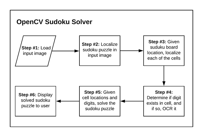
Creating an automatic sudoku puzzle solver with OpenCV is a 6-step process:

  • Step #1: Provide input image containing sudoku puzzle to our system.
  • Step #2: Locate where in the input image the puzzle is and extract the board.
  • Step #3: Given the board, locate each of the individual cells of the sudoku board (most standard sudoku puzzles are a 9×9 grid, so we’ll need to localize each of these cells).
  • Step #4: Determine if a digit exists in the cell, and if so, OCR it.
  • Step #5: Apply a sudoku puzzle solver/checker algorithm to validate the puzzle.
  • Step #6: Display the output result to the user.

The majority of these steps can be accomplished using OpenCV along with basic computer vision and image processing operations.

The biggest exception is Step #4, where we need to apply OCR.

OCR can be a bit tricky to apply, but we have a number of options:

  1. Use the Tesseract OCR engine, the de facto standard for open source OCR
  2. Utilize cloud-based OCR APIs, such as Microsoft Cognitive Services, Amazon Rekognition, or the Google Vision API
  3. Train our own custom OCR model

All of these are perfectly valid options; however, in order to make a complete end-to-end tutorial, I’ve decided that we’ll train our own custom sudoku OCR model using deep learning.

Be sure to strap yourself in — this is going to be a wild ride.

Configuring your development environment to solve sudoku puzzles with OpenCV and OCR

Figure 2: Our OpenCV and OCR sudoku solver uses a number of open source Python packages including TensorFlow/Keras, OpenCV, scikit-image, and scikit-learn.

To configure your system for this tutorial, I recommend following either of these tutorials to establish your baseline system and create a virtual environment:

Please note that PyImageSearch does not recommend or support Windows for CV/DL projects.

Once your environment is up and running, you’ll need another package for this tutorial. You need to install py-sudoku, the library we’ll be using to help us solve sudoku puzzles:

$ pip install py-sudoku

Project structure

Take a moment to grab today’s files from the “Downloads” section of this tutorial. From there, extract the archive, and inspect the contents:

$ tree --dirsfirst 
.
├── output
│   └── digit_classifier.h5
├── pyimagesearch
│   ├── models
│   │   ├── __init__.py
│   │   └── sudokunet.py
│   ├── sudoku
│   │   ├── __init__.py
│   │   └── puzzle.py
│   └── __init__.py
├── solve_sudoku_puzzle.py
├── sudoku_puzzle.jpg
└── train_digit_classifier.py

4 directories, 9 files

Inside, you’ll find a pyimagesearch module containing the following:

  • sudokunet.py: Holds the SudokuNet CNN architecture implemented with TensorFlow and Keras.
  • puzzle.py: Contains two helper utilities for finding the sudoku puzzle board itself as well as digits therein.

As with all CNNs, SudokuNet needs to be trained with data. Our train_digit_classifier.py script will train a digit OCR model on the MNIST dataset.

Once SudokuNet is successfully trained, we’ll deploy it with our solve_sudoku_puzzle.py script to solve a sudoku puzzle.

When your system is working, you can impress your friends with the app. Or better yet, fool them on the airplane as you solve puzzles faster than they possibly can in the seat right behind you! Don’t worry, I won’t tell!

SudokuNet: A digit OCR model implemented in Keras and TensorFlow

Every sudoku puzzle starts with an NxN grid (typically 9×9) where some cells are blank and other cells already contain a digit.

The goal is to use the knowledge about the existing digits to correctly infer the other digits.

But before we can solve sudoku puzzles with OpenCV, we first need to implement a neural network architecture that will handle OCR’ing the digits on the sudoku puzzle board — given that information, it will become trivial to solve the actual puzzle.

Fittingly, we’ll name our sudoku puzzle architecture SudokuNet.

Open up the sudokunet.py file in your pyimagesearch module, and insert the following code:

# import the necessary packages
from tensorflow.keras.models import Sequential
from tensorflow.keras.layers import Conv2D
from tensorflow.keras.layers import MaxPooling2D
from tensorflow.keras.layers import Activation
from tensorflow.keras.layers import Flatten
from tensorflow.keras.layers import Dense
from tensorflow.keras.layers import Dropout

All of SudokuNet‘s imports are from tf.keras. As you can see, we’ll be using Keras’ Sequential API as well as the layers shown.

Now that our imports are taken care of, let’s dive right into the implementation of our CNN:

class SudokuNet:
	@staticmethod
	def build(width, height, depth, classes):
		# initialize the model
		model = Sequential()
		inputShape = (height, width, depth)

Our SudokuNet class is defined with a single static method (no constructor) on Lines 10-12. The build method accepts the following parameters:

  • width: The width of an MNIST digit (28 pixels)
  • height: The height of an MNIST digit (28 pixels)
  • depth: Channels of MNIST digit images (1 grayscale channel)
  • classes: The number of digits 0-9 (10 digits)

Lines 14 and 15 initialize our model to be built with the Sequential API as well as establish the inputShape, which we’ll need for our first CNN layer.

Now that our model is initialized, let’s go ahead and build out our CNN:

		# first set of CONV => RELU => POOL layers
		model.add(Conv2D(32, (5, 5), padding="same",
			input_shape=inputShape))
		model.add(Activation("relu"))
		model.add(MaxPooling2D(pool_size=(2, 2)))

		# second set of CONV => RELU => POOL layers
		model.add(Conv2D(32, (3, 3), padding="same"))
		model.add(Activation("relu"))
		model.add(MaxPooling2D(pool_size=(2, 2)))

		# first set of FC => RELU layers
		model.add(Flatten())
		model.add(Dense(64))
		model.add(Activation("relu"))
		model.add(Dropout(0.5))

		# second set of FC => RELU layers
		model.add(Dense(64))
		model.add(Activation("relu"))
		model.add(Dropout(0.5))

		# softmax classifier
		model.add(Dense(classes))
		model.add(Activation("softmax"))

		# return the constructed network architecture
		return model

The body of our network is composed of:

  • CONV => RELU => POOL: Layer set 1
  • CONV => RELU => POOL: Layer set 2
  • FC => RELU: Fully-connected layer set with 50% dropout

The head of the network consists of a softmax classifier with the number of outputs being equal to the number of our classes (in our case: 10 digits).

Great job implementing SudokuNet!

If the CNN layers and working with the Sequential API was unfamiliar to you, I recommend checking out either of the following resources:

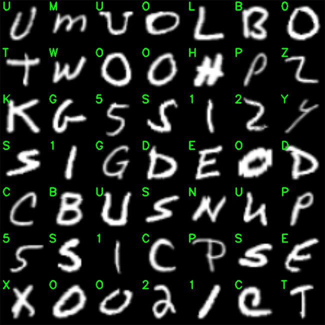
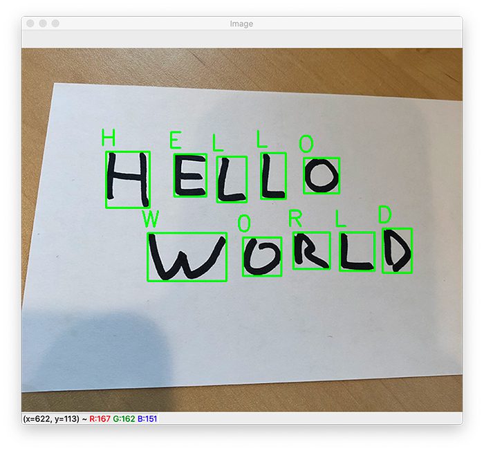
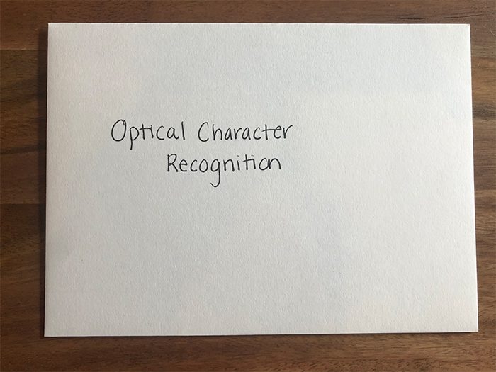
Note: As an aside, I’d like to take a moment to point out here that if you were, for example, building a CNN to classify 26 uppercase English letters plus the 10 digits (a total of 36 characters), you most certainly would need a deeper CNN (outside the scope of this tutorial, which focuses on digits as they apply to sudoku). I cover how to train networks on both digits and alphabet characters inside my book, OCR with OpenCV, Tesseract and Python.

Implementing our sudoku digit training script with Keras and TensorFlow

Figure 3: A sample of digits from Yann LeCun’s MNIST dataset of handwritten digits will be used to train a deep learning model to OCR/HWR handwritten digits with Keras/TensorFlow.

With the SudokuNet model architecture implemented, we can move on to creating a Python script that will train the model to recognize digits.

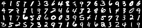
Perhaps unsurprisingly, we’ll be using the MNIST dataset to train our digit recognizer, as it fits quite nicely in this use case.

Open up the train_digit_classifier.py to get started:

# import the necessary packages
from pyimagesearch.models import SudokuNet
from tensorflow.keras.optimizers import Adam
from tensorflow.keras.datasets import mnist
from sklearn.preprocessing import LabelBinarizer
from sklearn.metrics import classification_report
import argparse

# construct the argument parser and parse the arguments
ap = argparse.ArgumentParser()
ap.add_argument("-m", "--model", required=True,
	help="path to output model after training")
args = vars(ap.parse_args())

We begin our training script with a small handful of imports. Most notably, we’re importing SudokuNet (discussed in the previous section) and the mnist dataset. The MNIST dataset of handwritten digits is built right into TensorFlow/Keras’ datasets module and will be cached to your machine on demand.

Our script requires a single command line argument: --model. When you execute the training script from the command line, simply pass a filename for your output model file (I recommend using the .h5 file extension).

Next, we’ll (1) set hyperparameters and (2) load and pre-process MNIST:

# initialize the initial learning rate, number of epochs to train
# for, and batch size
INIT_LR = 1e-3
EPOCHS = 10
BS = 128

# grab the MNIST dataset
print("[INFO] accessing MNIST...")
((trainData, trainLabels), (testData, testLabels)) = mnist.load_data()

# add a channel (i.e., grayscale) dimension to the digits
trainData = trainData.reshape((trainData.shape[0], 28, 28, 1))
testData = testData.reshape((testData.shape[0], 28, 28, 1))

# scale data to the range of [0, 1]
trainData = trainData.astype("float32") / 255.0
testData = testData.astype("float32") / 255.0

# convert the labels from integers to vectors
le = LabelBinarizer()
trainLabels = le.fit_transform(trainLabels)
testLabels = le.transform(testLabels)

You can configure training hyperparameters on Lines 17-19. Through experimentation, I’ve determined appropriate settings for the learning rate, number of training epochs, and batch size.

Note: Advanced users might wish to check out my Keras Learning Rate Finder tutorial to aid in automatically finding optimal learning rates.

To work with the MNIST digit dataset, we perform the following steps:

  • Load the dataset into memory (Line 23). This dataset is already split into training and testing data
  • Add a channel dimension to the digits to indicate that they are grayscale (Lines 30 and 31)
  • Scale data to the range of [0, 1] (Lines 30 and 31)
  • One-hot encode labels (Lines 34-36)

The process of one-hot encoding means that an integer such as 3 would be represented as follows:

[0, 0, 0, 1, 0, 0, 0, 0, 0, 0]

Or the integer 9 would be encoded like so:

[0, 0, 0, 0, 0, 0, 0, 0, 0, 1]

From here, we’ll go ahead and initialize and train SudokuNet on our digits data:

# initialize the optimizer and model
print("[INFO] compiling model...")
opt = Adam(lr=INIT_LR)
model = SudokuNet.build(width=28, height=28, depth=1, classes=10)
model.compile(loss="categorical_crossentropy", optimizer=opt,
	metrics=["accuracy"])

# train the network
print("[INFO] training network...")
H = model.fit(
	trainData, trainLabels,
	validation_data=(testData, testLabels),
	batch_size=BS,
	epochs=EPOCHS,
	verbose=1)

Lines 40-43 build and compile our model with the Adam optimizer and categorical cross-entropy loss.

Note: We’re focused on 10 digits. However, if you were only focused on recognizing binary numbers 0 and 1, then you would use loss="binary_crossentropy". Keep this in mind when working with two-class datasets or data subsets.

Training is launched via a call to the fit method (Lines 47-52).

Once training is complete, we’ll evaluate and export our model:

# evaluate the network
print("[INFO] evaluating network...")
predictions = model.predict(testData)
print(classification_report(
	testLabels.argmax(axis=1),
	predictions.argmax(axis=1),
	target_names=[str(x) for x in le.classes_]))

# serialize the model to disk
print("[INFO] serializing digit model...")
model.save(args["model"], save_format="h5")

Using our newly trained model, we make predictions on our testData (Line 56). From there we print a classification report to our terminal (Lines 57-60).

Finally, we save our model to disk (Line 64). Note that for TensorFlow 2.0+, we recommend explicitly setting the save_format="h5" (HDF5 format).

Training our sudoku digit recognizer with Keras and TensorFlow

We’re now ready to train our SudokuNet model to recognize digits.

Start by using the “Downloads” section of this tutorial to download the source code and example images.

From there, open up a terminal, and execute the following command:

$ python train_digit_classifier.py --model output/digit_classifier.h5
[INFO] accessing MNIST...
[INFO] compiling model...
[INFO] training network...
[INFO] training network...
Epoch 1/10
469/469 [==============================] - 22s 47ms/step - loss: 0.7311 - accuracy: 0.7530 - val_loss: 0.0989 - val_accuracy: 0.9706
Epoch 2/10
469/469 [==============================] - 22s 47ms/step - loss: 0.2742 - accuracy: 0.9168 - val_loss: 0.0595 - val_accuracy: 0.9815
Epoch 3/10
469/469 [==============================] - 21s 44ms/step - loss: 0.2083 - accuracy: 0.9372 - val_loss: 0.0452 - val_accuracy: 0.9854
...
Epoch 8/10
469/469 [==============================] - 22s 48ms/step - loss: 0.1178 - accuracy: 0.9668 - val_loss: 0.0312 - val_accuracy: 0.9893
Epoch 9/10
469/469 [==============================] - 22s 47ms/step - loss: 0.1100 - accuracy: 0.9675 - val_loss: 0.0347 - val_accuracy: 0.9889
Epoch 10/10
469/469 [==============================] - 22s 47ms/step - loss: 0.1005 - accuracy: 0.9700 - val_loss: 0.0392 - val_accuracy: 0.9889
[INFO] evaluating network...
              precision    recall  f1-score   support

           0       0.98      1.00      0.99       980
           1       0.99      1.00      0.99      1135
           2       0.99      0.98      0.99      1032
           3       0.99      0.99      0.99      1010
           4       0.99      0.99      0.99       982
           5       0.98      0.99      0.98       892
           6       0.99      0.98      0.99       958
           7       0.98      1.00      0.99      1028
           8       1.00      0.98      0.99       974
           9       0.99      0.98      0.99      1009

    accuracy                           0.99     10000
   macro avg       0.99      0.99      0.99     10000
weighted avg       0.99      0.99      0.99     10000

[INFO] serializing digit model...

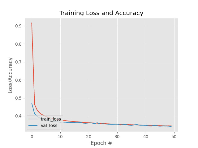
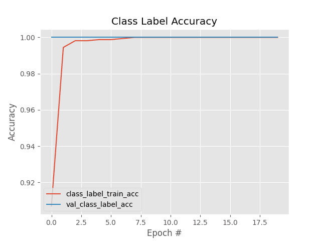
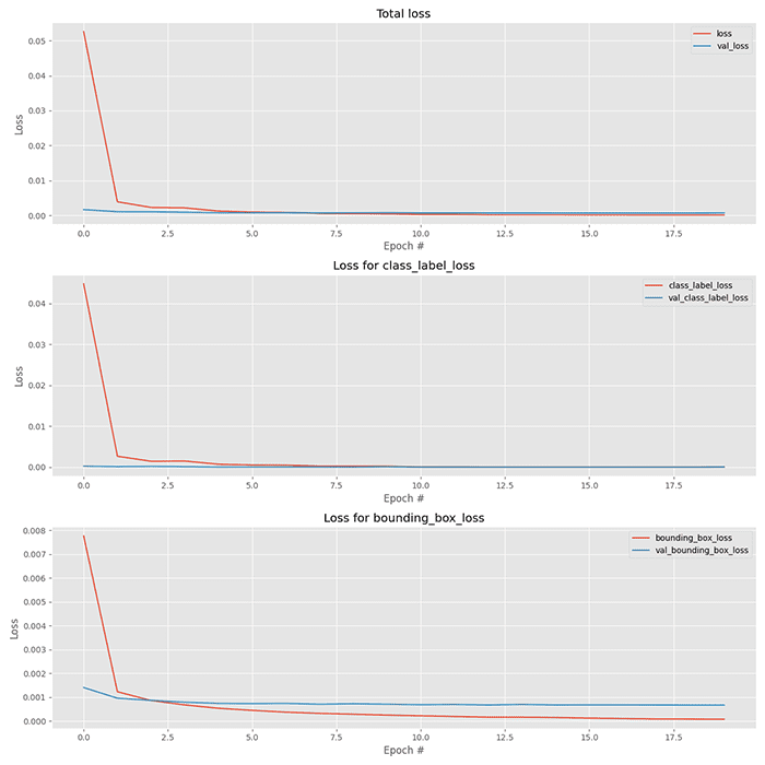
Here, you can see that our SudokuNet model has obtained 99% accuracy on our testing set.

You can verify that the model is serialized to disk by inspecting your output directory:

$ ls -lh output
total 2824
-rw-r--r--@ 1 adrian  staff   1.4M Jun  7 07:38 digit_classifier.h5

This digit_classifier.h5 file contains our Keras/TensorFlow model, which we’ll use to recognize the digits on a sudoku board later in this tutorial.

This model is quite small and could be deployed to a Raspberry Pi or even a mobile device such as an iPhone running the CoreML framework.

Finding the sudoku puzzle board in an image with OpenCV

At this point, we have a model that can recognize digits in an image; however, that digit recognizer doesn’t do us much good if it can’t locate the sudoku puzzle board in an image.

For example, let’s say we presented the following sudoku puzzle board to our system:

How are we going to locate the actual sudoku puzzle board in the image?

And once we’ve located the puzzle, how do we identify each of the individual cells?

To make our lives a bit easier, we’ll be implementing two helper utilities:

  • find_puzzle: Locates and extracts the sudoku puzzle board from the input image
  • extract_digit: Examines each cell of the sudoku puzzle board and extracts the digit from the cell (provided there is a digit)

This section will show you how to implement the find_puzzle method, while the next section will show the extract_digit implementation.

Open up the puzzle.py file in the pyimagesearch module, and we’ll get started:

# import the necessary packages
from imutils.perspective import four_point_transform
from skimage.segmentation import clear_border
import numpy as np
import imutils
import cv2

def find_puzzle(image, debug=False):
	# convert the image to grayscale and blur it slightly
	gray = cv2.cvtColor(image, cv2.COLOR_BGR2GRAY)
	blurred = cv2.GaussianBlur(gray, (7, 7), 3)

Our two helper functions require my imutils implementation of a four_point_transform for deskewing an image to obtain a bird’s eye view.

Additionally, we’ll use the clear_border routine in our extract_digit function to clean up the edges of a sudoku cell. Most operations will be driven with OpenCV with a little bit of help from NumPy and imutils.

Our find_puzzle function comes first and accepts two parameters:

  • image: The photo of a sudoku puzzle.
  • debug: A optional boolean indicating whether to show intermediate steps so you can better visualize what is happening under the hood of our computer vision pipeline. If you are encountering any issues, I recommend setting debug=True and using your computer vision knowledge to iron out any bugs.

Our first step is to convert our image to grayscale and apply a Gaussian blur operation with a 7×7 kernel (Lines 10 and 11).

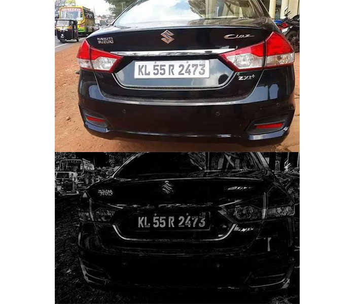
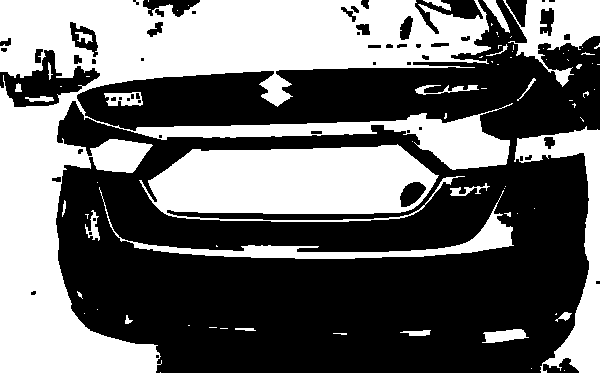
And next, we’ll apply adaptive thresholding:

	# apply adaptive thresholding and then invert the threshold map
	thresh = cv2.adaptiveThreshold(blurred, 255,
		cv2.ADAPTIVE_THRESH_GAUSSIAN_C, cv2.THRESH_BINARY, 11, 2)
	thresh = cv2.bitwise_not(thresh)

	# check to see if we are visualizing each step of the image
	# processing pipeline (in this case, thresholding)
	if debug:
		cv2.imshow("Puzzle Thresh", thresh)
		cv2.waitKey(0)

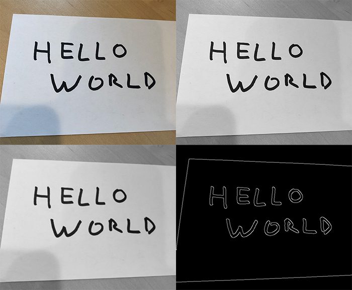
Binary adaptive thresholding operations allow us to peg grayscale pixels toward each end of the [0, 255] pixel range. In this case, we’ve both applied a binary threshold and then inverted the result as shown in Figure 5 below:

Figure 5: OpenCV has been used to perform a binary inverse threshold operation on the input image.

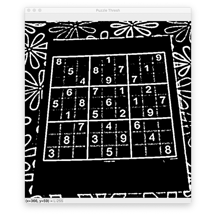
Just remember, you’ll only see something similar to the inverted thresholded image if you have your debug option set to True.

Now that our image is thresholded, let’s find and sort contours:

	# find contours in the thresholded image and sort them by size in
	# descending order
	cnts = cv2.findContours(thresh.copy(), cv2.RETR_EXTERNAL,
		cv2.CHAIN_APPROX_SIMPLE)
	cnts = imutils.grab_contours(cnts)
	cnts = sorted(cnts, key=cv2.contourArea, reverse=True)

	# initialize a contour that corresponds to the puzzle outline
	puzzleCnt = None

	# loop over the contours
	for c in cnts:
		# approximate the contour
		peri = cv2.arcLength(c, True)
		approx = cv2.approxPolyDP(c, 0.02 * peri, True)

		# if our approximated contour has four points, then we can
		# assume we have found the outline of the puzzle
		if len(approx) == 4:
			puzzleCnt = approx
			break

Here, we find contours and sort by area in reverse order (Lines 26-29).

One of our contours will correspond to the outline of the sudoku grid — puzzleCnt is initialized to None on Line 32. Let’s determine which of our cnts is our puzzleCnt using the following approach:

  • Loop over all contours beginning on Line 35
  • Determine the perimeter of the contour (Line 37)
  • Approximate the contour (Line 38)
  • Check if contour has four vertices, and if so, mark it as the puzzleCnt, and break out of the loop (Lines 42-44)

It is possible that the outline of the sudoku grid isn’t found. In that case, let’s raise an Exception:

	# if the puzzle contour is empty then our script could not find
	# the outline of the sudoku puzzle so raise an error
	if puzzleCnt is None:
		raise Exception(("Could not find sudoku puzzle outline. "
			"Try debugging your thresholding and contour steps."))

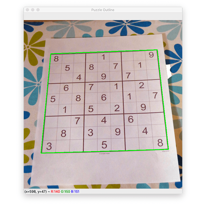
	# check to see if we are visualizing the outline of the detected
	# sudoku puzzle
	if debug:
		# draw the contour of the puzzle on the image and then display
		# it to our screen for visualization/debugging purposes
		output = image.copy()
		cv2.drawContours(output, [puzzleCnt], -1, (0, 255, 0), 2)
		cv2.imshow("Puzzle Outline", output)
		cv2.waitKey(0)

If the sudoku puzzle is not found, we raise an Exception to tell the user/developer what happened (Lines 48-50).

And again, if we are debugging, we’ll visualize what is going on under the hood by drawing the puzzle contour outline on the image, as shown in Figure 6:

Figure 6: The border of the sudoku puzzle board is found by means of determining the largest contour with four points using OpenCV’s contour operations.

With the contour of the puzzle in hand (fingers crossed), we’re then able to deskew the image to obtain a top-down bird’s eye view of the puzzle:

	# apply a four point perspective transform to both the original
	# image and grayscale image to obtain a top-down bird's eye view
	# of the puzzle
	puzzle = four_point_transform(image, puzzleCnt.reshape(4, 2))
	warped = four_point_transform(gray, puzzleCnt.reshape(4, 2))

	# check to see if we are visualizing the perspective transform
	if debug:
		# show the output warped image (again, for debugging purposes)
		cv2.imshow("Puzzle Transform", puzzle)
		cv2.waitKey(0)

	# return a 2-tuple of puzzle in both RGB and grayscale
	return (puzzle, warped)

Applying a four-point perspective transform effectively deskews our sudoku puzzle grid, making it much easier for us to determine rows, columns, and cells as we move forward (Lines 65 and 66). This operation is performed on the original RGB image and gray image.

The final result of our find_puzzle function is shown in Figure 7:

Figure 7: After applying a four-point perspective transform using OpenCV, we’re left with a top-down bird’s eye view of the sudoku puzzle. At this point, we can begin working on finding characters and performing deep learning based OCR with TensorFlow/Keras.

Our find_puzzle return signature consists of a 2-tuple of the original RGB image and grayscale image after all operations, including the final four-point perspective transform.

Great job so far!

Let’s continue our forward march toward solving sudoku puzzles. Now we need a means to extract digits from sudoku puzzle cells, and we’ll do just that in the next section.

Extracting digits from a sudoku puzzle with OpenCV

Figure 8: The 
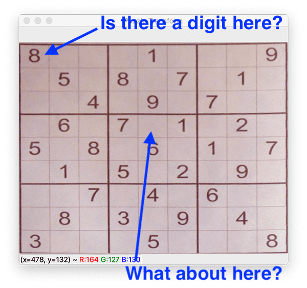
extract_digit helper function will help us find and extract digits or determine that a cell is empty and no digit is present. Each of these two cases is equally important for solving a sudoku puzzle. In the case where a digit is present, we need to OCR it.

In our previous section, you learned how to detect and extract the sudoku puzzle board from an image with OpenCV.

This section will show you how to examine each of the individual cells in a sudoku board, detect if there is a digit in the cell, and if so, extract the digit.

Continuing where we left off in the previous section, let’s open the puzzle.py file once again and get to work:

def extract_digit(cell, debug=False):
	# apply automatic thresholding to the cell and then clear any
	# connected borders that touch the border of the cell
	thresh = cv2.threshold(cell, 0, 255,
		cv2.THRESH_BINARY_INV | cv2.THRESH_OTSU)[1]
	thresh = clear_border(thresh)

	# check to see if we are visualizing the cell thresholding step
	if debug:
		cv2.imshow("Cell Thresh", thresh)
		cv2.waitKey(0)

Here, you can see we’ve defined our extract_digit function to accept two parameters:

  • cell: An ROI representing an individual cell of the sudoku puzzle (it may or may not contain a digit)
  • debug: A boolean indicating whether intermediate step visualizations should be shown to your screen

Our first step, on Lines 80-82, is to threshold and clear any foreground pixels that are touching the borders of the cell (such as any line markings from the cell dividers). The result of this operation can be shown via Lines 85-87.

Let’s see if we can find the digit contour:

	# find contours in the thresholded cell
	cnts = cv2.findContours(thresh.copy(), cv2.RETR_EXTERNAL,
		cv2.CHAIN_APPROX_SIMPLE)
	cnts = imutils.grab_contours(cnts)

	# if no contours were found than this is an empty cell
	if len(cnts) == 0:
		return None

	# otherwise, find the largest contour in the cell and create a
	# mask for the contour
	c = max(cnts, key=cv2.contourArea)
	mask = np.zeros(thresh.shape, dtype="uint8")
	cv2.drawContours(mask, [c], -1, 255, -1)

Lines 90-92 find the contours in the thresholded cell. If no contours are found, we return None (Lines 95 and 96).

Given our contours, cnts, we then find the largest contour by pixel area and construct an associated mask (Lines 100-102).

From here, we’ll continue working on trying to isolate the digit in the cell:

	# compute the percentage of masked pixels relative to the total
	# area of the image
	(h, w) = thresh.shape
	percentFilled = cv2.countNonZero(mask) / float(w * h)

	# if less than 3% of the mask is filled then we are looking at
	# noise and can safely ignore the contour
	if percentFilled < 0.03:
		return None

	# apply the mask to the thresholded cell
	digit = cv2.bitwise_and(thresh, thresh, mask=mask)

	# check to see if we should visualize the masking step
	if debug:
		cv2.imshow("Digit", digit)
		cv2.waitKey(0)

	# return the digit to the calling function
	return digit

Dividing the pixel area of our mask by the area of the cell itself (Lines 106 and 107) gives us the percentFilled value (i.e., how much our cell is “filled up” with white pixels). Given this percentage, we ensure the contour is not simply “noise” (i.e., a very small contour).

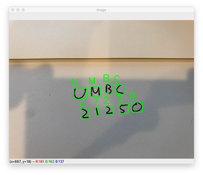
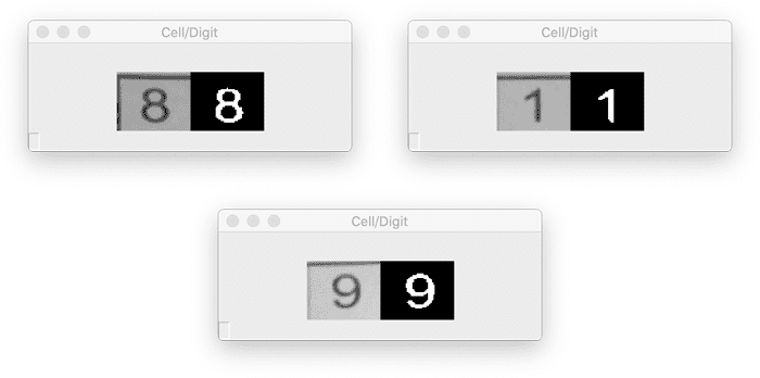
Assuming we don’t have a noisy cell, Line 115 applies the mask to the thresholded cell. This mask is optionally shown on screen (Lines 118-120) and is finally returned to the caller. Three example results are shown in Figure 9:

Figure 9: A few examples, which demonstrate the original warped cell (left) and the result of pre-processing the cell to obtain the digit mask (right).

Great job implementing the digit extraction pipeline!

Implementing our OpenCV sudoku puzzle solver

At this point, we’re armed with the following components:

  • Our custom SudokuNet model trained on the MNIST dataset of digits and residing on disk ready for use
  • A means to extract the sudoku puzzle board and apply a perspective transform
  • A pipeline to extract digits within individual cells of the sudoku puzzle or ignore ones that we consider to be noise
  • The py-sudoku puzzle solver installed in our Python virtual environment, which saves us from having to engineer an algorithm from hand and lets us focus solely on the computer vision challenge

We are now ready to put each of the pieces together to build a working OpenCV sudoku solver!

Open up the solve_sudoku_puzzle.py file, and let’s complete our sudoku solver project:

# import the necessary packages
from pyimagesearch.sudoku import extract_digit
from pyimagesearch.sudoku import find_puzzle
from tensorflow.keras.preprocessing.image import img_to_array
from tensorflow.keras.models import load_model
from sudoku import Sudoku
import numpy as np
import argparse
import imutils
import cv2

# construct the argument parser and parse the arguments
ap = argparse.ArgumentParser()
ap.add_argument("-m", "--model", required=True,
	help="path to trained digit classifier")
ap.add_argument("-i", "--image", required=True,
	help="path to input sudoku puzzle image")
ap.add_argument("-d", "--debug", type=int, default=-1,
	help="whether or not we are visualizing each step of the pipeline")
args = vars(ap.parse_args())

As with nearly all Python scripts, we have a selection of imports to get the party started.

These include our custom computer vision helper functions: extract_digit and find_puzzle. We’ll be using TensorFlow/Keras’ load_model method to grab our trained SudokuNet model from disk and load it into memory.

The sudoku import is made possible by py-sudoku, which we’ve previously installed; at this stage, this is the most foreign import for us computer vision and deep learning nerds.

Let’s define three command line arguments:

  • --model: The path to our trained digit classifier generated while following the instructions in the “Training our sudoku digit recognizer with Keras and TensorFlow” section
  • --image: Your path to a sudoku puzzle photo residing on disk (for simplicity, we won’t be interacting with a camera or accepting REST API calls today, although I encourage you to do so on your own time)
  • --debug: A flag indicating whether to show intermediate pipeline step debugging visualizations

As we’re now equipped with imports and our args dictionary, let’s load both our (1) digit classifier model and (2) input --image from disk:

# load the digit classifier from disk
print("[INFO] loading digit classifier...")
model = load_model(args["model"])

# load the input image from disk and resize it
print("[INFO] processing image...")
image = cv2.imread(args["image"])
image = imutils.resize(image, width=600)

From there, we’ll find our puzzle and prepare to isolate the cells therein:

# find the puzzle in the image and then
(puzzleImage, warped) = find_puzzle(image, debug=args["debug"] > 0)

# initialize our 9x9 sudoku board
board = np.zeros((9, 9), dtype="int")

# a sudoku puzzle is a 9x9 grid (81 individual cells), so we can
# infer the location of each cell by dividing the warped image
# into a 9x9 grid
stepX = warped.shape[1] // 9
stepY = warped.shape[0] // 9

# initialize a list to store the (x, y)-coordinates of each cell
# location
cellLocs = []

Here, we:

  • Find the sudoku puzzle in the input --image via our find_puzzle helper (Line 32)
  • Initialize our sudoku board — a 9×9 array (Line 35)
  • Infer the step size for each of the cells by simple division (Lines 40 and 41)
  • Initialize a list to hold the (x, y)-coordinates of cell locations (Line 45)

And now, let’s begin a nested loop over rows and columns of the sudoku board:

# loop over the grid locations
for y in range(0, 9):
	# initialize the current list of cell locations
	row = []

	for x in range(0, 9):
		# compute the starting and ending (x, y)-coordinates of the
		# current cell
		startX = x * stepX
		startY = y * stepY
		endX = (x + 1) * stepX
		endY = (y + 1) * stepY

		# add the (x, y)-coordinates to our cell locations list
		row.append((startX, startY, endX, endY))

Accounting for every cell in the sudoku puzzle, we loop over rows (Line 48) and columns (Line 52) in a nested fashion.

Inside, we use our step values to determine the starting and ending (x, y)-coordinates of the current cell (Lines 55-58).

Line 61 appends the coordinates as a tuple to this particular row. Each row will have nine entries (9x 4-tuples).

Now we’re ready to crop out the cell and recognize the digit therein (if one is present):

		# crop the cell from the warped transform image and then
		# extract the digit from the cell
		cell = warped[startY:endY, startX:endX]
		digit = extract_digit(cell, debug=args["debug"] > 0)

		# verify that the digit is not empty
		if digit is not None:
			# resize the cell to 28x28 pixels and then prepare the
			# cell for classification
			roi = cv2.resize(digit, (28, 28))
			roi = roi.astype("float") / 255.0
			roi = img_to_array(roi)
			roi = np.expand_dims(roi, axis=0)

			# classify the digit and update the sudoku board with the
			# prediction
			pred = model.predict(roi).argmax(axis=1)[0]
			board[y, x] = pred

	# add the row to our cell locations
	cellLocs.append(row)

Step by step, we proceed to:

  • Crop the cell from transformed image and then extract the digit (Lines 65 and 66)

  • If the digit is not None, then we know there is an actual digit in the cell (rather than an empty space), at which point we:

    • Pre-process the digit roi in the same manner that we did for training (Lines 72-75)
    • Classify the digit roi with SudokuNet (Line 79)
    • Update the sudoku puzzle board array with the predicted value of the cell (Line 80)
  • Add the row‘s (x, y)-coordinates to the cellLocs list (Line 83) — the last line of our nested loop over rows and columns

And now, let’s solve the sudoku puzzle with py-sudoku:

# construct a sudoku puzzle from the board
print("[INFO] OCR'd sudoku board:")
puzzle = Sudoku(3, 3, board=board.tolist())
puzzle.show()

# solve the sudoku puzzle
print("[INFO] solving sudoku puzzle...")
solution = puzzle.solve()
solution.show_full()

As you can see, first, we display the sudoku puzzle board as it was interpreted via OCR (Lines 87 and 88).

Then, we make a call to puzzle.solve to solve the sudoku puzzle (Line 92). And again, this is where the py-sudoku package does the mathematical algorithm to solve our puzzle.

We go ahead and print out the solved puzzle in our terminal (Line 93)

And of course, what fun would this project be if we didn’t visualize the solution on the puzzle image itself? Let’s do that now:

# loop over the cell locations and board
for (cellRow, boardRow) in zip(cellLocs, solution.board):
	# loop over individual cell in the row
	for (box, digit) in zip(cellRow, boardRow):
		# unpack the cell coordinates
		startX, startY, endX, endY = box

		# compute the coordinates of where the digit will be drawn
		# on the output puzzle image
		textX = int((endX - startX) * 0.33)
		textY = int((endY - startY) * -0.2)
		textX += startX
		textY += endY

		# draw the result digit on the sudoku puzzle image
		cv2.putText(puzzleImage, str(digit), (textX, textY),
			cv2.FONT_HERSHEY_SIMPLEX, 0.9, (0, 255, 255), 2)

# show the output image
cv2.imshow("Sudoku Result", puzzleImage)
cv2.waitKey(0)

To annotate our image with the solution numbers, we simply:

  • Loop over cell locations and the board (Lines 96-98)
  • Unpack cell coordinates (Line 100)
  • Compute coordinates of where text annotation will be drawn (Lines 104-107)
  • Draw each output digit on our puzzle board photo (Lines 110 and 111)
  • Display our solved sudoku puzzle image (Line 114) until any key is pressed (Line 115)

Nice job!

Let’s kick our project into gear in the next section. You’ll be very impressed with your hard work!

OpenCV sudoku puzzle solver OCR results

We are now ready to put our OpenV sudoku puzzle solver to the test!

Make sure you use the “Downloads” section of this tutorial to download the source code, trained digit classifier, and example sudoku puzzle image.

From there, open up a terminal, and execute the following command:

$ python solve_sudoku_puzzle.py --model output/digit_classifier.h5 \
	--image sudoku_puzzle.jpg
[INFO] loading digit classifier...
[INFO] processing image...
[INFO] OCR'd sudoku board:
+-------+-------+-------+
| 8     |   1   |     9 |
|   5   | 8   7 |   1   |
|     4 |   9   | 7     |
+-------+-------+-------+
|   6   | 7   1 |   2   |
| 5   8 |   6   | 1   7 |
|   1   | 5   2 |   9   |
+-------+-------+-------+
|     7 |   4   | 6     |
|   8   | 3   9 |   4   |
| 3     |   5   |     8 |
+-------+-------+-------+

[INFO] solving sudoku puzzle...

---------------------------
9x9 (3x3) SUDOKU PUZZLE
Difficulty: SOLVED
---------------------------
+-------+-------+-------+
| 8 7 2 | 4 1 3 | 5 6 9 |
| 9 5 6 | 8 2 7 | 3 1 4 |
| 1 3 4 | 6 9 5 | 7 8 2 |
+-------+-------+-------+
| 4 6 9 | 7 3 1 | 8 2 5 |
| 5 2 8 | 9 6 4 | 1 3 7 |
| 7 1 3 | 5 8 2 | 4 9 6 |
+-------+-------+-------+
| 2 9 7 | 1 4 8 | 6 5 3 |
| 6 8 5 | 3 7 9 | 2 4 1 |
| 3 4 1 | 2 5 6 | 9 7 8 |
+-------+-------+-------+
Figure 10: You’ll have to resist the temptation to say “Bingo!” (wrong game) when you achieve this solved sudoku puzzle result using OpenCV, OCR, and TensorFlow/Keras.

As you can see, we have successfully solved the sudoku puzzle using OpenCV, OCR, and deep learning!

And now, if you’re the betting type, you could challenge a friend or significant other to see who can solve 10 sudoku puzzles the fastest on your next transcontinental airplane ride! Just don’t get caught snapping a few photos!

Credits

This tutorial was inspired by Aakash Jhawar and by Part 1 and Part 2 of his sudoku puzzle solver.

Additionally, you’ll note that I used the same example sudoku puzzle board that Aakash did, not out of laziness, but to demonstrate how the same puzzle can be solved with different computer vision and image processing techniques.

I really enjoyed Aakash’s articles and recommend PyImageSearch readers check them out as well (especially if you want to implement a sudoku solver from scratch rather than using the py-sudoku library).

What’s next?

Optical Character Recognition (OCR), OpenCV, and Tesseract
Figure 11: If you’re ready to solve your next OCR challenge, you’ll love my upcoming OCR Book. Click here to stay informed about my latest project!

Today, we learned how to solve a fun sudoku puzzle using OCR techniques spanning from training a deep learning model to creating a couple of image processing pipelines.

When you go to tackle any computer vision project, you need to know what’s possible and how to break a project down into achievable milestones.

But for a lot of readers of my blog that e-mail me daily, a single project is very daunting.

You wonder:

  • Where on Earth do I begin?
  • How do I get from point A to point B? Or what is point A in the first place?
  • What’s possible, and what isn’t?
  • Which tools do I need, and how can I use them effectively?
  • How can I get from my “BIG idea” to my “working solution” faster?

You’re not alone!

Your coach, mentor, or teacher has probably told you that “practice makes perfect” or “study harder.” And they are not wrong.

I’ll add that “studying smarter” is part of the equation too. I’ve learned not to focus on theory when I’m learning something new (such as OCR). Instead, I like to solve problems and learn by doing. By studying a new topic this way, I’m more successful at producing measurable results than if I were to remember complex equations.

If you want to study Optical Character Recognition (OCR) the smart way, look no further than my upcoming book.

Inside, you’ll find plenty of examples that are directly applicable to your OCR challenge.

Readers of mine tend to resonate with my no-nonsense and no mathematical fluff style of teaching in my books and courses. Grab one today, and get started.

Or hold out for my new OCR-specific book, which is in the planning and early development stages right now. If you want to stay in the loop, simply click here and fill in your information:

Summary

In this tutorial, you learned how to implement a sudoku puzzle solver using OpenCV, deep learning, and OCR.

In order to find and locate the sudoku puzzle board in the image, we utilized OpenCV and basic image processing techniques, including blurring, thresholding, and contour processing, just to name a few.

To actually OCR the digits on the sudoku board, we trained a custom digit recognition model using Keras and TensorFlow.

Combining the sudoku board locator with our digit OCR model allowed us to make quick work of solving the actual sudoku puzzle.

If you’re interested in learning more about OCR, I’m authoring a brand-new book called Optical Character Recognition with OpenCV, Tesseract, and Python.

To learn more about the book (and be notified when it launches at the exclusive discounted price), just click here, and enter your email address.

Otherwise, to download the source code to this post (and be notified when future tutorials are published here on PyImageSearch), simply enter your email address in the form below!

Download the Source Code and FREE 17-page Resource Guide

Enter your email address below to get a .zip of the code and a FREE 17-page Resource Guide on Computer Vision, OpenCV, and Deep Learning. Inside you’ll find my hand-picked tutorials, books, courses, and libraries to help you master CV and DL!

The post OpenCV Sudoku Solver and OCR appeared first on PyImageSearch.


My OCR with OpenCV, Tesseract, and Python IndieGoGo campaign will go live on Wednesday, August 19th at 10AM EDT

$
0
0

BIG news to share today!

I’m so incredibly excited to announce that my OCR with Tesseract, OpenCV, and Python IndieGoGo campaign is set to launch in exactly one week on Wednesday, August 19th at 10AM EDT.

So, why am I writing a book on OCR?

  • Despite all the advances in deep learning, OCR is still incredibly challenging.
  • Tools like Tesseract are cumbersome, hard to use, and provide few tutorials or documentation
  • And not to mention, integrating OCR and Tesseract into your own OpenCV projects can leave you pulling out your hair (I should know, I’m bald).

My new book demystifies OCR, allowing you to successfully and confidently apply OCR to your work, school projects, and research.

What will be covered in the book?

My new OCR book:

  • Covers the Tesseract OCR engine
  • Shows you how to tune all the knobs and dials of Tersseract to improve OCR accuracy
  • Teaches you how to integrate Tesseract with OpenCV in your own projects
  • Provides chapters on training custom OCR models from scratch
  • Utilizes deep learning to create OCR models on your own custom datasets
  • Shows you how to use cloud-based OCR APIs, such as Amazon Rekognition, Microsoft Cognitive Services, and the Google Vision API

Additionally, I’ve included a number of case studies on:

  • Building an OpenCV Sudoku solver
  • OCR’ing a form document such as an invoice, resume etc.
  • Creating a receipt scanner
  • Building an Automatic License/Number Plate (ANPR) system with OCR
  • How to apply OCR to video streams
  • How to improve OCR speed with your GPU
  • Training a Tesseract model from scratch
  • How to use Keras and TensorFlow to train custom OCR models
  • and more!

Certificate of Completion

This book will include a Certificate of Completion option. After successfully completing the quizzes and assignments for each lesson in the book, you will be awarded a certificate of completion which you can included on your LinkedIn profile, resume, etc.

Why IndieGoGo? Didn’t you use Kickstarter for previous campaigns?

Long-time PyImageSearch readers will note that I’ve launched three crowdfunding campaigns in the past (one for the PyImageSearch Gurus course, one for Deep Learning for Computer Vision with Python, and another for Raspberry Pi for Computer Vision). All three of these were launched using Kickstarter, a popular crowdfunding platform.

That raises the question — why use IndieGoGo over Kickstarter?

There are two reasons:

First, the Kickstarter platform is buggy. I’ve reported a number of bugs to Kickstarter over the past four years using their platform. These bugs were never fixed. And to be totally candid, I’ve started to lose a bit of faith in Kickstarter.

But more importantly, Kickstarter makes it confusing to offer multiple discounts and deals. When I ran the Kickstarter campaign for Raspberry Pi for Computer Vision, the single biggest point of feedback was that the checkout process was confusing.

IndieGoGo has a much more intuitive, straightforward checkout process, allowing you to:

  1. Grab your copy of OCR with OpenCV, Tesseract, and Python at the exclusive pre-launch pricing
  2. Additionally purchase copies of my other books and courses at discounted rates (if you choose)

My goal is to make it as easy as possible for you to take advantage of these deals and discounts — and when I tested the IndieGoGo platform, it was a no-brainer.

I was afraid to fail.

Back in February 2015, I launched my very first Kickstarter crowdfunding campaign. This campaign was for the PyImageSearch Gurus course, which has now become the best course online to learn computer vision, deep learning, and OpenCV.

But let me tell you, that Kickstarter campaign almost never launched.

No one knows this, but back in November 2014, the startup I was working for lost our funding. We had a government contract with the State of Maryland, and when the state election resulted in the governorship changing hands, the governor-elect canceled our contract immediately.

Here I was, fresh out of graduate school, PhD diploma in hand, and I was already out of work!

I was at a critical juncture at that point in my life; I could go out, find a new job, and continue on the same pathor, I could figure out a way to make PyImageSearch my full-time job.

I chose the latter.

I put my back against the wall and hunkered down for what I knew would be a fight for my life.

I knew the blows were coming. I felt like Rocky Balboa fighting Apollo Creed…but if I could withstand the punches, I could succeed.

But let me tell you, a punch is still a punch — and it hurts.

Bills were piling up. I had just moved in with my girlfriend (who would become my wife, a few years later). I was up against the ropes. I had my mitts up to protect my head, but I was taking body blow after body blow. If my hands were to fall, I knew I was out — I couldn’t take a punch to the head.

Leading up to the PyImageSearch Kickstarter campaign I was a nervous wreck. I barely slept in the four nights before it launched.

I was jittery and anxious. My left eye was twitching. I had constant catastrophic “what if” thoughts:

  • What if I can’t pay my bills?
  • What if I go broke?
  • I just moved in with this girl that I love — what if she leaves me because this career decision doesn’t work out?

What I failed to realize, but what I know now, is regardless of whether the PyImageSearch Gurus course was a success or not, I was still going to wake up the next morning. Life was going to continue.

  • If it was a success, great! I would have clear stepping stones to running PyImageSearch full-time.
  • And if it failed, at least I learned something. Yeah, life would be a bit harder for 6-12 months as I found a new job and paid back debt, but realistically, I was only 24 at the time. I had more than enough time in my life to recover from that punch.

Too often I see developers, students, and researchers convincing themselves not to learn a new skill because they are afraid of failing.

I learned something from that Kickstarter campaign six years ago — the biggest failure on my part would have been not to launch it.

If I would have given in to my fear of failure and pulled the plug at the last minute, then the PyImageSearch Gurus course wouldn’t exist.

And if that course didn’t exist, well, it’s very likely that PyImageSearch wouldn’t exist either. The success of that course brought in the students and the money necessary to grow PyImageSearch to what it is today.

In my opinion, the only true failure is failing to invest in yourself physically, mentally, and educationally.

  • Invest in your body, it’s the only one you have. It needs to last you 70+ years. Workout often, eat healthy, and drink lots of water. Learn to reduce (or eliminate) alcohol and caffeine consumption. Get 8 hours of sleep every night.
  • Invest in your mind and keep it sharp. Meditate before bed and first thing in the morning. Utilize a daily gratitude journal. Let go of your ego and apologize when you hurt another people’s feelings (even if you know you were right and justified). And most importantly, celebrate the people in your life that mean the most to you. Put them on a pedestal and make them feel wanted, special, and remarkable.
  • Invest in your education, it’s what keeps you young (literally). Studies in neuroplasticity (i.e., your brain’s ability to modify connections and rewire itself) show that stimulation via education helps reduce the risk of dementia, Alzheimer’s disease, and other brain degeneration conditions. Even if you are older and retired, you still need to learn to keep that brain young! And if you’re younger, there’s simply no excuse for not investing in yourself and your education — it’s important not only for your career, but for your long-term health.

What’s next?

OCR is one of the most challenging sub-fields of computer vision and deep learning. While a simple, intuitive concept, OCR has still yet to be “fully solved”. No off-the-shelf OCR package exists that is 100% accurate and works in every use case/situation.

My book will teach you how to successfully and confidently apply OCR to your own work, projects, and research. I guarantee that. Please consider joining me and grabbing your copy of my new book at the exclusive discounted rates.

The IndieGoGo campaign will launch next week, on Wednesday, August 19th at 10AM EDT. You’ll be able to claim your copy at the exclusive pre-launch prices then.

I’ll be back tomorrow with a sneak preview of the book.

Join the PyImageSearch Newsletter and Grab My FREE 17-page Resource Guide PDF

Enter your email address below to join the PyImageSearch Newsletter and download my FREE 17-page Resource Guide PDF on Computer Vision, OpenCV, and Deep Learning.

The post My OCR with OpenCV, Tesseract, and Python IndieGoGo campaign will go live on Wednesday, August 19th at 10AM EDT appeared first on PyImageSearch.

Sneak preview: OCR with OpenCV, Tesseract, and Python

$
0
0

Wow, the IndieGoGo launch date of Wednesday, August 19th is approaching so fast!

I still have a ton of work left to do and I’m currently neck-deep in IndieGoGo campaign logistics, but I took a few minutes and recorded this sneak peak preview of OCR with OpenCV, Tesseract, and Python:

The video is just under six minutes and covers all the details on the IndieGoGo campaign — I recommend you watch the video overview if you have any interest in this OCR book.

That said, I understand and respect that you’re busy and might not have the time to watch the video, so I’ve included the high-level bullet points below:

  • 0m15s: OCR is a simple concept — we take an input image, automatically recognize the text in the image, and then convert it to a machine-encoded variable
  • 0m30s: But despite being such an intuitive concept, OCR is extremely challenging. The field of CV has existed for over 50 years but we still have not solved OCR
  • 0m45s: Trying to code custom OCR software is near impossible. And utilizing OCR engines such as Tesseract can be challenging if you don’t know which knobs and dials to tune
  • 1m20s: Deep learning is responsible for unprecedented accuracy in computer vision — but which models, layer types, and loss functions do you use for OCR?
  • 2m00s: This book will teach you how to successfully (and confidently) apply OCR to your work, research, and projects
  • 2m15s: I discuss and demo the OCR projects you will learn inside the text, including OCR basics, text detection, automatically OCR’ing documents/forms, training custom OCR models with Tesseract, ANPR, handwriting recognition, OCR in video, and more!
  • 3m40s: Since this book covers such a large amount of content, I’ve decided to break the book down into three volumes, called “bundles”. You’ll be able to choose a bundle based on how in-depth you want to study OCR, which projects/chapters interest you the most, along with your particular budget.
  • 4m10s: I show what chapters are included in each bundle.
  • 5m47s: OCR is extremely hard, but my new book un-weaves all the complexity for you and gives you a clear, easy to follow path to successfully apply OCR to your own work.

How you educate yourself defines your character.

This past Saturday morning I finished reading Erik Larson’s Issac’s Storm, the true story of how a powerful hurricane absolutely destroyed the town of Galveston, Texas in 1900.

This storm is considered to be deadliest hurricane in United States history, not just because of the storm’s raw power, but because of man’s arrogance at the turn of the century — forecasters believed that they could not only predict the weather, but control it as well.

Mother nature has a way of knocking us down a few pegs and keeping our hubris in check.

One of my favorite quotes from the book is where Larson paraphrases Hippocrates, a prominent Greek physician who lived around 400 BC:

Hippocrates believed climate determined the character of men and nations.

It makes sense if you think about it.

  • If the weather is too hot, your fields can’t grow
  • If it’s too cold, your your crops will freeze and die
  • If it rains too much, your town will flood
  • And if it’s too windy, your house will blow over

It’s hard to build a great nation when the weather prevents you from finding food, shelter, or employment!

However, I personally believe it’s education, not climate, that determines the character of men and nations.

  • Education is how we grow, not only as individuals, but collectively as well.
  • Exposing ourselves to new concepts opens our minds and makes us more accepting of things we didn’t previously understand or couldn’t relate to
  • Education requires a level of discipline, and within that discipline we build character
  • The final product of routine daily education is enlightenment — and it takes enlightened people to build a strong nation

I have a passion for education. Every day I allocate one hour to educating myself on a topic I don’t know much about. I then spend the rest of the day educating PyImageSearch readers (such as yourself), teaching them how to successfully apply computer vision, deep learning, and OpenCV to their own projects.

Now, I’ll be teaching Optical Character Recognition. I hope you’ll consider grabbing a copy of my new book next week (or, at the very least, spend some time educating yourself on a new topic — education defines your character after all).

What’s next?

Like I said, if you have the time, the sneak preview video is definitely worth the watch. The video goes into more depth than what I can in this email, explaining what’s covered in the book and how it’s organized.

I hope that you decide to support the OCR with OpenCV, Tesseract, and Python IndieGoGo campaign on Wednesday, August 19th at 10AM EDT — if you’re ready to learn how to successfully apply OCR to your projects, then this is the perfect book for you!

To be notified when more IndieGoGo announcements go live (including ones I won’t be publishing on this blog), be sure to signup for the OCR with OpenCV, Tesseract, and Python notification list!

Join the PyImageSearch Newsletter and Grab My FREE 17-page Resource Guide PDF

Enter your email address below to join the PyImageSearch Newsletter and download my FREE 17-page Resource Guide PDF on Computer Vision, OpenCV, and Deep Learning.

The post Sneak preview: OCR with OpenCV, Tesseract, and Python appeared first on PyImageSearch.

Table of Contents – OCR with OpenCV, Tesseract, and Python

$
0
0

A few days ago I mentioned that on Wednesday, August 19th at 10AM EDT I am launching an IndieGoGo crowdfunding campaign for my new book, OCR with OpenCV, Tesseract, and Python.

Today I’m going to share with you:

  • The Table of Contents to the book
  • Additional details on how the book is structured
  • What is included in the book, including source code, pre-configured VM, access to the private community forums, etc.
  • The Certificate of Completion you’ll be awarded after completing all quizzes/exams associated with the text

Let’s dive in!

What is this book?

OCR with OpenCV, Tesseract, and Python will teach you how to successfully apply Optical Character Recognition to your work, projects, and research.

You will learn via practical, hands-on projects (with lots of code) so you can not only develop your own OCR Projects, but feel confident while doing so.

Inside the book we will focus on:

  • Getting started with OCR
  • Learning the basics of the Tesseract OCR engine
  • Discovering how to improve OCR accuracy using Tesseract options and configurations
  • Interfacing with Tesseract via the Python programming language
  • Localizing and detecting text in images using both OpenCV and Tesseract
  • Using OpenCV and image processing techniques to improve OCR accuracy
  • Using machine learning to denoise our images for better OCR accuracy
  • Image/document registration and alignment to build an invoice scanning project
  • Training our own custom deep learning models with Keras and TensorFlow
  • Solving Sudoku puzzles with OCR, OpenCV, and Keras/TensorFlow
  • Automatic License/Number Plate Recognition (ANPR)
  • Handwriting recognition
  • Performing OCR in real-time video streams
  • Utilizing GPUs for faster OCR inference
  • Using OCR engines in the cloud, including Amazon Rekognition, Microsoft Cognitive Services, and the Google Vison API
  • Tips, suggestions, and best practices when performing OCR

Currently I have 35+ chapters planned out, with more to come!

How is this book structured?

Since we’ll be covering so many OCR techniques in-depth, I’ve decided to break the book down into three volumes called “bundles”.

I’ve included a short breakdown of the three bundles below:

The “Intro to OCR” Bundle is right for you if:

  • You are new to the world of OCR and Computer Vision
  • You are just testing the OCR waters
  • You are on a budget

Inside this bundle you will learn the fundamentals of Optical Character Recognition using Tesseract, OpenCV, and Python. And while this is the lowest tier bundle, you’ll still be getting a great education with a lot of hands-on experience.

A full list of chapter topics follows:

  • Introduction
  • What is Optical Character Recognition (OCR)?
  • Tools, libraries, and packages for OCR
  • Installing our OCR libraries and tools
  • Your first OCR example with Tesseract
  • Detecting digits with Tesseract
  • Whitelisting and blacklisting characters with Tesseract
  • Determining and correcting text orientation with Tesseract
  • OCR’ing text and translating to different languages
  • Using Tesseract with non-English languages
  • Improving OCR accuracy with Tesseract Page Segmentation Modes (PSMs)
  • Improving OCR results with OpenCV and image processing
  • Utilizing spellchecking with OCR
  • OCR’ing passports using computer vision
  • Using OpenCV and template matching to OCR characters
  • OCR’ing characters with basic computer vision and image processing
  • Text bounding box localization and OCR with Tesseract
  • Rotated text bounding box localization with OpenCV
  • A complete text detection and OCR pipeline
  • Conclusions

The chapters inside the “Intro to OCR” Bundle will give you a strong foundation to build upon. For a more in-depth treatment of OCR, I would recommend either the “OCR Practitioner” Bundle or “OCR Expert” Bundle.

My Recommendation: The “Intro to OCR” Bundle is a great first step towards applying OCR to real-world projects. You’ll learn the fundamentals of OCR and Tesseract, empowering you to apply OCR to your own projects.

That said, if you are going with this bundle because you’re new to the world of computer vision and OCR, then you should absolutely look at the Practical Python and OpenCV and PyImageSearch Gurus add-ons. Both of these can be used to help you level-up your computer vision skills quickly (and be more successful when applying OCR).

The “OCR Practitioner” Bundle builds on the previous bundle and includes every chapter in the “Intro to OCR” Bundle. This bundle is geared towards more advanced OCR algorithms, techniques, and use cases, including deep learning, image/document alignment, OCR in real-time video streams, OCR with GPUs, cloud-based OCR APIs, and more!

Not only will you be getting every chapter in the “Intro to OCR” Bundle, but you’ll also receive the following:

  • Introduction
  • Training custom OCR models with Keras and TensorFlow
  • Using machine learning to denoise images for better OCR accuracy
  • Image and document registration
  • Automatically aligning and OCR’ing a document, invoice, form, etc.
  • Building an OpenCV Sudoku solver using OCR
  • OCR’ing receipts
  • Automatic License/Number Plate Recognition with OCR
  • Text blur detection
  • OCR’ing real-time video streams
  • Improving text detection speed with OpenCV and GPUs
  • Handwriting recognition
  • Text detection and OCR with the Amazon Rekognition API
  • Using the Microsoft Cognitive Services API for OCR
  • OCR with the Google Vision API
  • Training custom Tesseract OCR models
  • Fine-tuning Tesseract OCR models
  • Utilizing the EasyOCR package for fast, efficient OCR
  • Conclusions

My Recommendation: The “OCR Practitioner Bundle” gives you the best bang for your buck. You should choose this bundle if you want a super in-depth treatment of OCR, but cannot afford the “OCR Expert” Bundle.

If you’re new to computer vision and deep learning, I highly suggest you also get the PyImageSearch Gurus and/or Deep Learning for Computer Vision with Python add-ons — both of these resources will teach you computer vision and deep learning quickly (ensuring you get more value out of your purchase of the OCR book).

The “OCR Expert” Bundle includes everything from both the “Intro to OCR” Bundle and “OCR Practitioner” Bundle.

It also includes:

  • All bonus chapters from stretch goals during the IndieGoGo campaign (including chapters that are authored after the campaign has ended).
  • A physical, printed edition of all three volumes of OCR with OpenCV, Tesseract, and Pythonthis is the only bundle that includes a hardcopy edition.
  • Access to my private community forums for additional help and support. You’ll get faster, more detailed answers to your questions and you’ll be able to better connect with myself and other readers. (again, the other two bundles do not have access to these forums).
  • A Certificate of Completion upon successfully completing all lessons and quizzes associated with the text.

My Recommendation: You should go with the “OCR Expert” Bundle if (1) you want to study OCR in-depth and (2) you want additional help and support along the way. When it comes to learning Optical Character Recognition, you just can’t beat this bundle!

Additionally, the “OCR Expert” Bundle includes a Certificate of Completion. To receive the certificate, you will need to complete all lessons and quizzes associated with the text.

After successfully completing all lessons/quizzes, you will receive your certificate and be able to embed it directly on your LinkedIn profile, thereby demonstrating your Optical Character Recognition skills.

What’s next?

There you have it — the complete Table of Contents for OCR with OpenCV, Tesseract, and Python. I hope after looking over this list you’re excited as I am!

I also have some secret bonus chapters that I’m keeping under wraps until the IndieGoGo launches. Stay tuned for this details.

To be notified when more IndieGoGo announcements go live (including ones I won’t be publishing on this blog), be sure to signup for the OCR with OpenCV, Tesseract, and Python notification list!

Join the PyImageSearch Newsletter and Grab My FREE 17-page Resource Guide PDF

Enter your email address below to join the PyImageSearch Newsletter and download my FREE 17-page Resource Guide PDF on Computer Vision, OpenCV, and Deep Learning.

The post Table of Contents – OCR with OpenCV, Tesseract, and Python appeared first on PyImageSearch.

OCR with Keras, TensorFlow, and Deep Learning

$
0
0

In this tutorial, you will learn how to train an Optical Character Recognition (OCR) model using Keras, TensorFlow, and Deep Learning. This post is the first in a two-part series on OCR with Keras and TensorFlow:

  • Part 1: Training an OCR model with Keras and TensorFlow (today’s post)
  • Part 2: Basic handwriting recognition with Keras and TensorFlow (next week’s post)

For now, we’ll primarily be focusing on how to train a custom Keras/TensorFlow model to recognize alphanumeric characters (i.e., the digits 0-9 and the letters A-Z).

Building on today’s post, next week we’ll learn how we can use this model to correctly classify handwritten characters in custom input images.

The goal of this two-part series is to obtain a deeper understanding of how deep learning is applied to the classification of handwriting, and more specifically, our goal is to:

  • Become familiar with some well-known, readily available handwriting datasets for both digits and letters
  • Understand how to train deep learning model to recognize handwritten digits and letters
  • Gain experience in applying our custom-trained model to some real-world sample data
  • Understand some of the challenges with real-world noisy data and how we might want to augment our handwriting datasets to improve our model and results

We’ll be starting with the fundamentals of using well-known handwriting datasets and training a ResNet deep learning model on these data.

To learn how to train an OCR model with Keras, TensorFlow, and deep learning, just keep reading.

Looking for the source code to this post?

Jump Right To The Downloads Section

OCR with Keras, TensorFlow, and Deep Learning

In the first part of this tutorial, we’ll discuss the steps required to implement and train a custom OCR model with Keras and TensorFlow.

We’ll then examine the handwriting datasets that we’ll use to train our model.

From there, we’ll implement a couple of helper/utility functions that will aid us in loading our handwriting datasets from disk and then preprocessing them.

Given these helper functions, we’ll be able to create our custom OCR training script with Keras and TensorFlow.

After training, we’ll review the results of our OCR work.

Let’s get started!

Our deep learning OCR datasets

Figure 1: We are using two datasets for our OCR training with Keras and TensorFlow. On the left, we have the standard MNIST 0-9 dataset. On the right, we have the Kaggle A-Z dataset from Sachin Patel, which is based on the NIST Special Database 19.

In order to train our custom Keras and TensorFlow model, we’ll be utilizing two datasets:

The standard MNIST dataset is built into popular deep learning frameworks, including Keras, TensorFlow, PyTorch, etc. A sample of the MNIST 0-9 dataset can be seen in Figure 1 (left). The MNIST dataset will allow us to recognize the digits 0-9. Each of these digits is contained in a 28 x 28 grayscale image. You can read more about MNIST here.

But what about the letters A-Z? The standard MNIST dataset doesn’t include examples of the characters A-Zhow are we going to recognize them?

The answer is to use the NIST Special Database 19, which includes A-Z characters. This dataset actually covers 62 ASCII hexadecimal characters corresponding to the digits 0-9, capital letters A-Z, and lowercase letters a-z.

To make the dataset easier to use, Kaggle user Sachin Patel has released the dataset in an easy to use CSV file. This dataset takes the capital letters A-Z from NIST Special Database 19 and rescales them to be 28 x 28 grayscale pixels to be in the same format as our MNIST data.

For this project, we will be using just the Kaggle A-Z dataset, which will make our preprocessing a breeze. A sample of it can be seen in Figure 1 (right).

We’ll be implementing methods and utilities that will allow us to:

  1. Load both the datasets for MNIST 0-9 digits and Kaggle A-Z letters from disk
  2. Combine these datasets together into a single, unified character dataset
  3. Handle class label skew/imbalance from having a different number of samples per character
  4. Successfully train a Keras and TensorFlow model on the combined dataset
  5. Plot the results of the training and visualize the output of the validation data

Configuring your OCR development environment

To configure your system for this tutorial, I first recommend following either of these tutorials:

Either tutorial will help you configure your system with all the necessary software for this blog post in a convenient Python virtual environment.

Project structure

Let’s review the project structure.

Once you grab the files from the “Downloads” section of this article, you’ll be presented with the following directory structure:

$ tree --dirsfirst --filelimit 10
.
├── pyimagesearch
│   ├── az_dataset
│   │   ├── __init__.py
│   │   └── helpers.py
│   ├── models
│   │   ├── __init__.py
│   │   └── resnet.py
│   └── __init__.py
├── a_z_handwritten_data.csv
├── handwriting.model
├── plot.png
└── train_ocr_model.py

3 directories, 9 files

Once we unzip our download, we find that our ocr-keras-tensorflow/ directory contains the following:

  • pyimagesearch module: includes the sub-modules az_dataset for I/O helper files and models for implementing the ResNet deep learning architecture
  • a_z_handwritten_data.csv: contains the Kaggle A-Z dataset
  • handwriting.model: where the deep learning ResNet model is saved
  • plot.png: plots the results of the most recent run of training of ResNet
  • train_ocr_model.py: the main driver file for training our ResNet model and displaying the results

Now that we have the lay of the land, let’s dig into the I/O helper functions we will use to load our digits and letters.

Our OCR dataset helper functions

In order to train our custom Keras and TensorFlow OCR model, we first need to implement two helper utilities that will allow us to load both the Kaggle A-Z datasets and the MNIST 0-9 digits from disk.

These I/O helper functions are appropriately named:

  • load_az_dataset: for the Kaggle A-Z letters
  • load_mnist_dataset: for the MNIST 0-9 digits

They can be found in the helpers.py file of az_dataset submodules of pyimagesearch.

Let’s go ahead and examine this helpers.py file. We will begin with our import statements and then dig into our two helper functions: load_az_dataset and load_mnist_dataset.

# import the necessary packages
from tensorflow.keras.datasets import mnist
import numpy as np

Line 2 imports the MNIST dataset, mnist, which is now one of the standard datasets that conveniently comes with Keras in tensorflow.keras.datasets.

Next, let’s dive into load_az_dataset, the helper function to load the Kaggle A-Z letter data.

def load_az_dataset(datasetPath):
	# initialize the list of data and labels
	data = []
	labels = []

	# loop over the rows of the A-Z handwritten digit dataset
	for row in open(datasetPath):
		# parse the label and image from the row
		row = row.split(",")
		label = int(row[0])
		image = np.array([int(x) for x in row[1:]], dtype="uint8")

		# images are represented as single channel (grayscale) images
		# that are 28x28=784 pixels -- we need to take this flattened
		# 784-d list of numbers and repshape them into a 28x28 matrix
		image = image.reshape((28, 28))

		# update the list of data and labels
		data.append(image)
		labels.append(label)

Our function load_az_dataset takes a single argument datasetPath, which is the location of the Kaggle A-Z CSV file (Line 5). Then, we initialize our arrays to store the data and labels (Lines 7 and 8).

Each row in Sachin Patel’s CSV file contains 785 columns — one column for the class label (i.e., “A-Z”) plus 784 columns corresponding to the 28 x 28 grayscale pixels. Let’s parse it.

Beginning on Line 11, we are going to loop over each row of our CSV file and parse out the label and the associated image. Line 14 parses the label, which will be the integer label associated with a letter A-Z. For example, the letter “A” has a label corresponding to the integer “0” and the letter “Z” has an integer label value of “25”.

Next, Line 15 parses our image and casts it as a NumPy array of unsigned 8-bit integers, which correspond to the grayscale values for each pixel from [0, 255].

We reshape our image (Line 20) from a flat 784-dimensional array to one that is 28 x 28, corresponding to the dimensions of each of our images.

We will then append each image and label to our data and label arrays respectively (Lines 23 and 24).

To finish up this function, we will convert the data and labels to NumPy arrays and return the image data and labels:

	# convert the data and labels to NumPy arrays
	data = np.array(data, dtype="float32")
	labels = np.array(labels, dtype="int")

	# return a 2-tuple of the A-Z data and labels
	return (data, labels)

Presently, our image data and labels are just Python lists, so we are going to type cast them as NumPy arrays of float32 and int, respectively (Lines 27 and 28).

Nice job implementing our first function!

Our next I/O helper function, load_mnist_dataset, is considerably simpler.

def load_mnist_dataset():
	# load the MNIST dataset and stack the training data and testing
	# data together (we'll create our own training and testing splits
	# later in the project)
	((trainData, trainLabels), (testData, testLabels)) = mnist.load_data()
	data = np.vstack([trainData, testData])
	labels = np.hstack([trainLabels, testLabels])

	# return a 2-tuple of the MNIST data and labels
	return (data, labels)

Line 33 loads our MNIST 0-9 digit data using Keras’s helper function, mnist.load_data. Notice that we don’t have to specify a datasetPath like we did for the Kaggle data because Keras, conveniently, has this dataset built-in.

Keras’s mnist.load_data comes with a default split for training data, training labels, test data, and test labels. For now, we are just going to combine our training and test data for MNIST using np.vstack for our image data (Line 38) and np.hstack for our labels (Line 39).

Later, in train_ocr_model.py, we will be combining our MNIST 0-9 digit data with our Kaggle A-Z letters. At that point, we will create our own custom split of test and training data.

Finally, Line 42 returns the image data and associated labels to the calling function.

Congratulations! You have now completed the I/O helper functions to load both the digit and letter samples to be used for OCR and deep learning. Next, we will examine our main driver file used for training and viewing the results.

Training our OCR Model using Keras and TensorFlow

In this section, we are going to train our OCR model using Keras, TensorFlow, and a PyImageSearch implementation of the very popular and successful deep learning architecture, ResNet.

Remember to save your model for next week, when we will implement a custom solution for handwriting recognition.

To get started, locate our primary driver file, train_ocr_model.py, which is found in the main directory, ocr-keras-tensorflow/. This file contains a reference to a file resnet.py, which is located in the models/ sub-directory under the pyimagesearch module.

Note: Although we will not be doing a detailed walk-through of resnet.py in this blog, you can get a feel for the ResNet architecture with my blog post on Fine-tuning ResNet with Keras and Deep Learning. For more advanced details, please my see my book, Deep Learning for Computer Vision with Python.

Let’s take a moment to review train_ocr_model.py. Afterward, we will come back and break it down, step by step.

First, we’ll review the packages that we will import:

# set the matplotlib backend so figures can be saved in the background
import matplotlib
matplotlib.use("Agg")

# import the necessary packages
from pyimagesearch.models import ResNet
from pyimagesearch.az_dataset import load_mnist_dataset
from pyimagesearch.az_dataset import load_az_dataset
from tensorflow.keras.preprocessing.image import ImageDataGenerator
from tensorflow.keras.optimizers import SGD
from sklearn.preprocessing import LabelBinarizer
from sklearn.model_selection import train_test_split
from sklearn.metrics import classification_report
from imutils import build_montages
import matplotlib.pyplot as plt
import numpy as np
import argparse
import cv2

This is a long list of import statements, but don’t worry. It means we have a lot of packages that have already been written to make our lives much easier.

Starting off on Line 5, we will import matplotlib and set up the backend of it by writing the results to a file using matplotlib.use("Agg")(Line 6).

We then have some imports from our custom pyimagesearch module for our deep learning architecture and our I/O helper functions that we just reviewed:

  • We import ResNet from our pyimagesearch.model, which contains our own custom implementation of the popular ResNet deep learning architecture (Line 9).
  • Next, we import our I/O helper functions load_mnist_data (Line 10) and load_az_dataset (Line 11) from pyimagesearch.az_dataset.

We have a couple of imports from the Keras module of TensorFlow, which greatly simplify our data augmentation and training:

  • Line 12 imports ImageDataGenerator to help us efficiently augment our dataset.
  • We then import SGD, the popular Stochastic Gradient Descent (SGD) optimization algorithm (Line 13).

Following on, we import three helper functions from scikit-learn to help us label our data, split our testing and training data sets, and print out a nice classification report to show us our results:

  • To convert our labels from integers to a vector in what is called one-hot encoding, we import LabelBinarizer (Line 14).
  • To help us easily split out our testing and training data sets, we import train_test_split from scinkit-learn (Line 15).
  • From the metrics submodule, we import classification_report to print out a nicely formatted classification report (Line 16).

Next, we will use a custom package that I wrote called imutils.

From imutils, we import build_montages to help us build a montage from a list of images (Line 17). For more information on building montages, please refer to my Montages with OpenCV tutorial.

We will finally import Matplotlib (Line 18) and OpenCV (Line 21).

Now, let’s review our three command line arguments:

# construct the argument parser and parse the arguments
ap = argparse.ArgumentParser()
ap.add_argument("-a", "--az", required=True,
	help="path to A-Z dataset")th
ap.add_argument("-m", "--model", type=str, required=True,
	help="path to output trained handwriting recognition model")
ap.add_argument("-p", "--plot", type=str, default="plot.png",
	help="path to output training history file")
args = vars(ap.parse_args())

We have three arguments to review:

  • --az: The path to the Kaggle A-Z dataset (Lines 25 and 26)
  • --model: The path to output the trained handwriting recognition model (Lines 27 and 28)
  • --plot: The path to output the training history file (Lines 29 and 30)

So far, we have our imports, convenience function, and command line args ready to go. We have several steps remaining to set up the training for ResNet, compile it, and train it.

Now, we will set up the training parameters for ResNet and load our digit and letter data using the helper functions that we already reviewed:

# initialize the number of epochs to train for, initial learning rate,
# and batch size
EPOCHS = 50
INIT_LR = 1e-1
BS = 128

# load the A-Z and MNIST datasets, respectively
print("[INFO] loading datasets...")
(azData, azLabels) = load_az_dataset(args["az"])
(digitsData, digitsLabels) = load_mnist_dataset()

Lines 35-37 initialize the parameters for the training of our ResNet model.

Then, we load the data and labels for the Kaggle A-Z and MNIST 0-9 digits data, respectively (Lines 41 and 42), making use of the I/O helper functions that we reviewed at the beginning of the post.

Next, we are going to perform a number of steps to prepare our data and labels to be compatible with our ResNet deep learning model in Keras and TensorFlow:

# the MNIST dataset occupies the labels 0-9, so let's add 10 to every
# A-Z label to ensure the A-Z characters are not incorrectly labeled
# as digits
azLabels += 10

# stack the A-Z data and labels with the MNIST digits data and labels
data = np.vstack([azData, digitsData])
labels = np.hstack([azLabels, digitsLabels])

# each image in the A-Z and MNIST digts datasets are 28x28 pixels;
# however, the architecture we're using is designed for 32x32 images,
# so we need to resize them to 32x32
data = [cv2.resize(image, (32, 32)) for image in data]
data = np.array(data, dtype="float32")

# add a channel dimension to every image in the dataset and scale the
# pixel intensities of the images from [0, 255] down to [0, 1]
data = np.expand_dims(data, axis=-1)
data /= 255.0

As we combine our letters and numbers into a single character data set, we want to remove any ambiguity where there is overlap in the labels so that each label in the combined character set is unique.

Currently, our labels for A-Z go from [0, 25], corresponding to each letter of the alphabet. The labels for our digits go from 0-9, so there is overlap — which would be a problematic if we were to just combine them directly.

No problem! There is a very simple fix. We will just add ten to all of our A-Z labels so they all have integer label values greater than our digit label values (Line 47). Now, we have a unified labeling schema for digits 0-9 and letters A-Z without any overlap in the values of the labels.

Line 50 combines our data sets for our digits and letters into a single character dataset using np.vstack. Likewise, Line 51 unifies our corresponding labels for our digits and letters on using np.hstack.

Our ResNet architecture requires the images to have input dimensions of 32 x 32, but our input images currently have a size of 28 x 28. We resize each of the images using cv2.resize(Line 56).

We have two final steps to prepare our data for use with ResNet. On Line 61, we will add an extra “channel” dimension to every image in the dataset to make it compatible with the ResNet model in Keras/TensorFlow. Finally, we will scale our pixel intensities from a range of [0, 255] down to [0.0, 1.0] (Line 62).

Our next step is to prepare the labels for ResNet, weight the labels to account for the skew in the number of times each class (character) is represented in the data, and partition the data into test and training splits:

# convert the labels from integers to vectors
le = LabelBinarizer()
labels = le.fit_transform(labels)
counts = labels.sum(axis=0)

# account for skew in the labeled data
classTotals = labels.sum(axis=0)
classWeight = {}

# loop over all classes and calculate the class weight
for i in range(0, len(classTotals)):
	classWeight[i] = classTotals.max() / classTotals[i]

# partition the data into training and testing splits using 80% of
# the data for training and the remaining 20% for testing
(trainX, testX, trainY, testY) = train_test_split(data,
	labels, test_size=0.20, stratify=labels, random_state=42)

We instantiate a LabelBinarizer(Line 65), and then we convert the labels from integers to a vector of binaries with one-hot encoding (Line 66) using le.fit_transform. Lines 70-75 weight each class, based on the frequency of occurrence of each character. Next, we will use the scikit-learn train_test_split utility (Lines 79 and 80) to partition the data into 80% training and 20% testing.

From there, we’ll augment our data using an image generator from Keras:

# construct the image generator for data augmentation
aug = ImageDataGenerator(
	rotation_range=10,
	zoom_range=0.05,
	width_shift_range=0.1,
	height_shift_range=0.1,
	shear_range=0.15,
	horizontal_flip=False,
	fill_mode="nearest")

We can improve the results of our ResNet classifier by augmenting the input data for training using an ImageDataGenerator. Lines 82-90 include various rotations, scaling the size, horizontal translations, vertical translations, and tilts in the images. For more details on data augmentation, see our Keras ImageDataGenerator and Data Augmentation tutorial.

Now we are ready to initialize and compile the ResNet network:

# initialize and compile our deep neural network
print("[INFO] compiling model...")
opt = SGD(lr=INIT_LR, decay=INIT_LR / EPOCHS)
model = ResNet.build(32, 32, 1, len(le.classes_), (3, 3, 3),
	(64, 64, 128, 256), reg=0.0005)
model.compile(loss="categorical_crossentropy", optimizer=opt,
	metrics=["accuracy"])

Using the SGD optimizer and a standard learning rate decay schedule, we build our ResNet architecture (Lines 94-96). Each character/digit is represented as a 32×32 pixel grayscale image as is evident by the first three parameters to ResNet’s build method.

Note: For more details on ResNet, be sure to refer to the Practitioner Bundle of Deep Learning for Computer Vision with Python where you’ll learn how to implement and tune the powerful architecture.

Lines 97 and 98 compile our model with "categorical_crossentropy" loss and our established SGD optimizer. Please beware that if you are working with a 2-class only dataset (we are not), you would need to use the "binary_crossentropy" loss function.

Next, we will train the network, define label names, and evaluate the performance of the network:

# train the network
print("[INFO] training network...")
H = model.fit(
	aug.flow(trainX, trainY, batch_size=BS),
	validation_data=(testX, testY),
	steps_per_epoch=len(trainX) // BS,
	epochs=EPOCHS,
	class_weight=classWeight,
	verbose=1)

# define the list of label names
labelNames = "0123456789"
labelNames += "ABCDEFGHIJKLMNOPQRSTUVWXYZ"
labelNames = [l for l in labelNames]

# evaluate the network
print("[INFO] evaluating network...")
predictions = model.predict(testX, batch_size=BS)
print(classification_report(testY.argmax(axis=1),
	predictions.argmax(axis=1), target_names=labelNames))

We train our model using the model.fit method (Lines 102-108). The parameters are as follows:

  • aug.flow: establishes in-line data augmentation (Line 103)
  • validation_data: test input images (testX) and test labels (testY) (Line 104)
  • steps_per_epoch: how many batches are run per each pass of the full training data (Line 105)
  • epochs: the number of complete passes through the full data set during training (Line 106)
  • class_weight: weights due to the imbalance of data samples for various classes (e.g., digits and letters) in the training data (Line 107)
  • verbose: shows a progress bar during the training (Line 108)

Note: Formerly, TensorFlow/Keras required use of a method called .fit_generator in order to train a model using data generators (such as data augmentation objects). Now, the .fit method can handle generators/data augmentation as well, making for more-consistent code. This also applies to the migration from .predict_generator to .predict. Be sure to check out my articles about fit and fit_generator as well as data augmentation.

Next, we establish labels for each individual character. Lines 111-113 concatenates all of our digits and letters and form an array where each member of the array is a single digit or number.

In order to evaluate our model, we make predictions on the test set and print our classification report. We’ll see the report very soon in the next section!

Line 118 prints out the results using the convenient scikit-learn classification_report utility.

We will save the model to disk, plot the results of the training history, and save the training history:

# save the model to disk
print("[INFO] serializing network...")
model.save(args["model"], save_format="h5")

# construct a plot that plots and saves the training history
N = np.arange(0, EPOCHS)
plt.style.use("ggplot")
plt.figure()
plt.plot(N, H.history["loss"], label="train_loss")
plt.plot(N, H.history["val_loss"], label="val_loss")
plt.title("Training Loss and Accuracy")
plt.xlabel("Epoch #")
plt.ylabel("Loss/Accuracy")
plt.legend(loc="lower left")
plt.savefig(args["plot"])

As we have finished our training, we need to save the model comprised of the architecture and final weights. We will save our model, to disk, as a Hierarchical Data Format version 5 (HDF5) file, which is specified by the save_format (Line 123).

Next, we use matplotlib’s plt to generate a line plot for the training loss and validation set loss along with titles, labels for the axes, and a legend. The data for the training and validation losses come from the history of H, the results of model.fit from above with one point for every epoch (Lines 127-134). The plot of the training loss curves is saved to plot.png (Line 135).

Finally, let’s code our visualization procedure so we can see whether our model is working or not:

# initialize our list of output test images
images = []

# randomly select a few testing characters
for i in np.random.choice(np.arange(0, len(testY)), size=(49,)):
	# classify the character
	probs = model.predict(testX[np.newaxis, i])
	prediction = probs.argmax(axis=1)
	label = labelNames[prediction[0]]

	# extract the image from the test data and initialize the text
	# label color as green (correct)
	image = (testX[i] * 255).astype("uint8")
	color = (0, 255, 0)

	# otherwise, the class label prediction is incorrect
	if prediction[0] != np.argmax(testY[i]):
		color = (0, 0, 255)

	# merge the channels into one image, resize the image from 32x32
	# to 96x96 so we can better see it and then draw the predicted
	# label on the image
	image = cv2.merge([image] * 3)
	image = cv2.resize(image, (96, 96), interpolation=cv2.INTER_LINEAR)
	cv2.putText(image, label, (5, 20), cv2.FONT_HERSHEY_SIMPLEX, 0.75,
		color, 2)

	# add the image to our list of output images
	images.append(image)

# construct the montage for the images
montage = build_montages(images, (96, 96), (7, 7))[0]

# show the output montage
cv2.imshow("OCR Results", montage)
cv2.waitKey(0)

Line 138 initializes our array of test images.

Starting on Line 141, we randomly select 49 characters (to form a 7×7 grid) and proceed to:

  • Classify the character using our ResNet-based model (Lines 143-145)
  • Grab the individual character image from our test data (Line 149)
  • Set an annotation text color as green (correct) or red (incorrect) via Lines 150-154
  • Create a RGB representation of our single channel image and resize it for inclusion in our visualization montage (Lines 159 and 160)
  • Annotate the colored text label (Lines 161 and 162)
  • Add the image to our output images array (Line 165)

To close out, we assemble each annotated character image into an OpenCV Montage visualization grid, displaying the result until a key is pressed (Lines 168-172).

Congratulations! We learned a lot along the way! Next, we’ll see the results of our hard work.

Keras and TensorFlow OCR training results

Recall from the last section that our script (1) loads MNIST 0-9 digits and Kaggle A-Z letters, (2) trains a ResNet model on the dataset, and (3) produces a visualization so that we can ensure it is working properly.

In this section, we’ll execute our OCR model training and visualization script.

To get started, use the “Downloads” section of this tutorial to download the source code and datasets.

From there, open up a terminal, and execute the command below:

$ python train_ocr_model.py --az a_z_handwritten_data.csv --model handwriting.model
[INFO] loading datasets...
[INFO] compiling model...
[INFO] training network...
Epoch 1/50
2765/2765 [==============================] - 93s 34ms/step - loss: 0.9160 - accuracy: 0.8287 - val_loss: 0.4713 - val_accuracy: 0.9406
Epoch 2/50
2765/2765 [==============================] - 87s 31ms/step - loss: 0.4635 - accuracy: 0.9386 - val_loss: 0.4116 - val_accuracy: 0.9519
Epoch 3/50
2765/2765 [==============================] - 87s 32ms/step - loss: 0.4291 - accuracy: 0.9463 - val_loss: 0.3971 - val_accuracy: 0.9543
...
Epoch 48/50
2765/2765 [==============================] - 86s 31ms/step - loss: 0.3447 - accuracy: 0.9627 - val_loss: 0.3443 - val_accuracy: 0.9625
Epoch 49/50
2765/2765 [==============================] - 85s 31ms/step - loss: 0.3449 - accuracy: 0.9625 - val_loss: 0.3433 - val_accuracy: 0.9622
Epoch 50/50
2765/2765 [==============================] - 86s 31ms/step - loss: 0.3445 - accuracy: 0.9625 - val_loss: 0.3411 - val_accuracy: 0.9635
[INFO] evaluating network...
precision    recall  f1-score   support

           0       0.52      0.51      0.51      1381
           1       0.97      0.98      0.97      1575
           2       0.87      0.96      0.92      1398
           3       0.98      0.99      0.99      1428
           4       0.90      0.95      0.92      1365
           5       0.87      0.88      0.88      1263
           6       0.95      0.98      0.96      1375
           7       0.96      0.99      0.97      1459
           8       0.95      0.98      0.96      1365
           9       0.96      0.98      0.97      1392
           A       0.98      0.99      0.99      2774
           B       0.98      0.98      0.98      1734
           C       0.99      0.99      0.99      4682
           D       0.95      0.95      0.95      2027
           E       0.99      0.99      0.99      2288
           F       0.99      0.96      0.97       232
           G       0.97      0.93      0.95      1152
           H       0.97      0.95      0.96      1444
           I       0.97      0.95      0.96       224
           J       0.98      0.96      0.97      1699
           K       0.98      0.96      0.97      1121
           L       0.98      0.98      0.98      2317
           M       0.99      0.99      0.99      2467
           N       0.99      0.99      0.99      3802
           O       0.94      0.94      0.94     11565
           P       1.00      0.99      0.99      3868
           Q       0.96      0.97      0.97      1162
           R       0.98      0.99      0.99      2313
           S       0.98      0.98      0.98      9684
           T       0.99      0.99      0.99      4499
           U       0.98      0.99      0.99      5802
           V       0.98      0.99      0.98       836
           W       0.99      0.98      0.98      2157
           X       0.99      0.99      0.99      1254
           Y       0.98      0.94      0.96      2172
           Z       0.96      0.90      0.93      1215

    accuracy                           0.96     88491
   macro avg       0.96      0.96      0.96     88491
weighted avg       0.96      0.96      0.96     88491

[INFO] serializing network...

As you can see, our Keras/TensorFlow OCR model is obtaining ~96% accuracy on the testing set.

The training history can be seen below:

Figure 2: Here’s a plot of our training history. It shows little signs of overfitting, implying that our Keras and TensorFlow model is performing well on our OCR task.

As evidenced by the plot, there are few signs of overfitting, implying that our Keras and TensorFlow model is performing well at our basic OCR task.

Let’s take a look at some sample output from our testing set:

Figure 3: We can see from our sample output that our Keras and TensorFlow OCR model is performing quite well in identifying our character set.

As you can see, our Keras/TensorFlow OCR model is performing quite well!

And finally, if you check your current working directory, you should find a new file named handwriting.model:

$ ls *.model
handwriting.model

This file is is our serialized Keras and TensorFlow OCR model — we’ll be using it in next week’s tutorial on handwriting recognition.

Applying our OCR model to handwriting recognition

Figure 4: Next week, we will extend this tutorial to handwriting recognition.

At this point, you’re probably thinking:

Hey Adrian,

It’s pretty cool that we trained a Keras/TensorFlow OCR model — but what good does it do just sitting on my hard drive?

How can I use it to make predictions and actually recognize handwriting?

Rest assured, that very question will be addressed in next week’s tutorial — stay tuned; you won’t want to miss it!

What’s next?

Optical Character Recognition (OCR), OpenCV, and Tesseract
Figure 5: Did you enjoy learning how to train a custom OCR model using Keras and TensorFlow? Then you’ll love my upcoming book, Optical Character Recognition (OCR), OpenCV, and Tesseract. Click here to stay informed on book progress, launch dates, and exclusive discounts.

Optical Character Recognition (OCR) is a simple concept but is hard in practice: Create a piece of software that accepts an input image, have that software automatically recognize the text in the image, and then convert it to machine-encoded text (i.e., a “string” data type).

But despite being such an intuitive concept, OCR is incredibly hard. The field of computer vision has existed for over 50 years (with mechanical OCR machines dating back over 100 years), but we still have not “solved” OCR and created an off-the-shelf OCR system that works in nearly any situation.

And worse, trying to code custom software that can perform OCR is even harder:

  • Open source OCR packages like Tesseract can be difficult to use if you are new to the world of OCR.
  • Obtaining high accuracy with Tesseract typically requires that you know which options, parameters, and configurations to use — and unfortunately there aren’t many high-quality Tesseract tutorials or books online.
  • Computer vision and image processing libraries such as OpenCV and scikit-image can help you preprocess your images to improve OCR accuracy … but which algorithms and techniques do you use?
  • Deep learning is responsible for unprecedented accuracy in nearly every area of computer science. Which deep learning models, layer types, and loss functions should you be using for OCR?

If you’ve ever found yourself struggling to apply OCR to a project, or if you’re simply interested in learning OCR, my brand-new book, OCR with OpenCV, Tesseract, and Python is for you.

Regardless of your current experience level with computer vision and OCR, after reading this book, you will be armed with the knowledge necessary to tackle your own OCR projects.

If you’re interested in OCR, already have OCR project ideas/need for it at your company, or simply want to stay informed about our progress as we develop the book, please click the button below to stay informed. I’ll be sharing more with you soon!

Summary

In this tutorial, you learned how to train a custom OCR model using Keras and TensorFlow.

Our model was trained to recognize alphanumeric characters including the digits 0-9 as well as the letters A-Z. Overall, our Keras and TensorFlow OCR model was able to obtain ~96% accuracy on our testing set.

In next week’s tutorial, you’ll learn how to take our trained Keras/TensorFlow OCR model and use it for handwriting recognition on custom input images.

To download the source code to this post (and be notified when future tutorials are published here on PyImageSearch), simply enter your email address in the form below!

Download the Source Code and FREE 17-page Resource Guide

Enter your email address below to get a .zip of the code and a FREE 17-page Resource Guide on Computer Vision, OpenCV, and Deep Learning. Inside you’ll find my hand-picked tutorials, books, courses, and libraries to help you master CV and DL!

The post OCR with Keras, TensorFlow, and Deep Learning appeared first on PyImageSearch.

OCR: Handwriting recognition with OpenCV, Keras, and TensorFlow

$
0
0

In this tutorial, you will learn how to perform OCR handwriting recognition using OpenCV, Keras, and TensorFlow.

This post is Part 2 in our two-part series on Optical Character Recognition with Keras and TensorFlow:

As you’ll see further below, handwriting recognition tends to be significantly harder than traditional OCR that uses specific fonts/characters.

The reason this concept is so challenging is that unlike computer fonts, there are nearly infinite variations of handwriting styles. Every one of us has a personal style that is specific and unique.

My wife, for example, has amazing penmanship. Her handwriting is not only legible, but it’s stylized in a way that you would think a professional calligrapher wrote it:

Figure 1: My wife has the most beautiful penmanship.

Me on the other hand … my handwriting looks like someone crossed a doctor with a deranged squirrel:

Figure 2: As you can see, my handwriting leaves a little bit to be desired.

It’s barely legible. I’m often asked by those who read my handwriting at least 2-3 clarifying questions as to what a specific word or phrase is. And on more than one occasion, I’ve had to admit that I couldn’t read them either.

Talk about embarrassing! Truly, it’s a wonder they ever let me out of grade school.

These variations in handwriting styles pose quite a problem for Optical Character Recognition engines, which are typically trained on computer fonts, not handwriting fonts.

And worse, handwriting recognition is further complicated by the fact that letters can “connect” and “touch” each other, making it incredibly challenging for OCR algorithms to separate them, ultimately leading to incorrect OCR results.

Handwriting recognition is arguably the “holy grail” of OCR. We’re not there yet, but with the help of deep learning, we’re making tremendous strides.

Today’s tutorial will serve as an introduction to handwriting recognition. You’ll see examples of where handwriting recognition has performed well and other examples where it has failed to correctly OCR a handwritten character. I truly think you’ll find value in reading the rest of this handwriting recognition guide.

To learn how to perform handwriting recognition with OpenCV, Keras, and TensorFlow, just keep reading.

Looking for the source code to this post?

Jump Right To The Downloads Section

OCR: Handwriting recognition with OpenCV, Keras, and TensorFlow

In the first part of this tutorial, we’ll discuss handwriting recognition and how it’s different from “traditional” OCR.

I’ll then provide a brief review of the process for training our recognition model using Keras and TensorFlow — we’ll be using this trained model to OCR handwriting in this tutorial.

Note: If you haven’t read last week’s post, I strongly suggest you do so now before continuing, as this post outlines the model that we trained to OCR alphanumeric samples. You should have a firm understanding of the concepts and scripts from last week as a prerequisite for this tutorial.

We’ll review our project structure and then implement a Python script to perform handwriting recognition with OpenCV, Keras, and TensorFlow.

To wrap up today’s OCR tutorial, we’ll discuss our handwriting recognition results, including what worked and what didn’t.

What is handwriting recognition? And how is handwriting recognition different from traditional OCR?

Figure 3: OCR is more difficult for handwriting than for typed text. But why is it so difficult?

Traditional OCR algorithms and techniques assume we’re working with a fixed font of some sort. In the early 1900s, that could have been the font used by microfilms.

In the 1970s, specialized fonts were developed specifically for OCR algorithms, thereby making them more accurate.

By the 2000s, we could use the fonts that came pre-installed on our computers to automatically generate training data and use these fonts to train our OCR models.

Each of these fonts had something in common:

  1. They were engineered in some manner.
  2. There was a predictable and assumed space between each character (thereby making segmentation easier).
  3. The styles of the fonts were more conducive to OCR.

Essentially, engineered/computer-generated fonts make OCR far easier.

Handwriting recognition is an entirely different beast though. Consider the extreme amount of variations and how characters often overlap. Everyone has their own unique writing style.

Characters can be elongated, swooped, slanted, stylized, crunched, connected, tiny, gigantic, etc. (and come in any of these combinations).

Digitizing handwriting recognition is extremely challenging and is still far from solved — but deep learning is helping us improve our handwriting recognition accuracy.

Handwriting recognition – what we’ve done so far

Figure 4: Here we have our two datasets from last week’s post for OCR training with Keras and TensorFlow. On the left, we have the standard MNIST 0-9 dataset. On the right, we have the Kaggle A-Z dataset from Sachin Patel, which is based on the NIST Special Database 19.

In last week’s tutorial, we used Keras and TensorFlow to train a deep neural network to recognize both digits (0-9) and alphabetic characters (A-Z).

To train our network to recognize these sets of characters, we utilized the MNIST digits dataset as well as the NIST Special Database 19 (for the A-Z characters).

Our model obtained 96% accuracy on the testing set for handwriting recognition.

Today, we will learn how to use this model for handwriting recognition in our own custom images.

Configuring your OCR development environment

If you have not already configured TensorFlow and the associated libraries from last week’s tutorial, I first recommend following the relevant tutorial below:

The tutorials above will help you configure your system with all the necessary software for this blog post in a convenient Python virtual environment.

Project structure

If you haven’t yet, go to the “Downloads” section of this blog post and grab both the code and dataset for today’s tutorial.

Inside, you’ll find the following:

$ tree --dirsfirst --filelimit 10
.
└── ocr-handwriting-recognition
    ├── images
    │   ├── hello_world.png
    │   ├── umbc_address.png
    │   └── umbc_zipcode.png
    ├── pyimagesearch
    │   ├── az_dataset
    │   │   ├── __init__.py
    │   │   └── helpers.py
    │   ├── models
    │   │   ├── __init__.py
    │   │   └── resnet.py
    │   └── __init__.py
    ├── a_z_handwritten_data.csv
    ├── handwriting.model
    ├── ocr_handwriting.py
    ├── plot.png
    └── train_ocr_model.py

5 directories, 13 files

Once we unzip our download, we find that our ocr-handwriting-recognition/ directory contains the following:

  • pyimagesearch module:
    • Includes the sub-modules az_dataset for I/O helper functions and models for implementing the ResNet deep learning model
  • a_z_handwritten_data.csv: A CSV file that contains the Kaggle A-Z dataset
  • train_ocr_model.py: The main Python driver file from last week that we used to train our ResNet model and display our results. Our model and training plot files include:
    • handwriting.model: The custom OCR ResNet model we created in last week’s tutorial
    • plot.png: A plot of the results of our most recent OCR training run
  • images/ sub-directory: Contains three PNG test files for us to OCR with our Python driver script
  • ocr_handwriting.py: The main Python script for this week that we will use to OCR our handwriting samples

With the exception of ocr_handwriting.py and our new PNG files in images/, all of this should look very familiar from our tutorial from last week.

Now that we have a handle on the project structure, let’s dive into our new script.

Implementing our handwriting recognition OCR script with OpenCV, Keras, and TensorFlow

Let’s open up ocr_handwriting.py and review it, starting with the imports and command line arguments:

# import the necessary packages
from tensorflow.keras.models import load_model
from imutils.contours import sort_contours
import numpy as np
import argparse
import imutils
import cv2

# construct the argument parser and parse the arguments
ap = argparse.ArgumentParser()
ap.add_argument("-i", "--image", required=True,
	help="path to input image")
ap.add_argument("-m", "--model", type=str, required=True,
	help="path to trained handwriting recognition model")
args = vars(ap.parse_args())

Line 2 imports the load_model utility, which allows us to easily load the OCR model that we developed last week.

Using my imutils package, we then import sort_contours (Line 3) and imutils (Line 6), to facilitate operations with contours and resizing images.

Our command line arguments include:

  • --image: Our input image path (Lines 11 and 12)
  • --model: The path to our trained handwriting recognition model (Lines 13 and 14)

Next, we will load our custom handwriting OCR model that we developed in last week’s tutorial:

# load the handwriting OCR model
print("[INFO] loading handwriting OCR model...")
model = load_model(args["model"])

The load_model utility from Keras and TensorFlow makes it super simple to load our serialized handwriting recognition model (Line 19). Recall that our OCR model uses the ResNet deep learning architecture to classify each character corresponding to a digit 0-9 or a letter A-Z.

Note: For more details on the ResNet CNN architecture, please refer to the Deep Learning for Computer Vision with Python Practitioner Bundle.

Since we’ve loaded our model from disk, let’s grab our image, pre-process it, and find character contours:

# load the input image from disk, convert it to grayscale, and blur
# it to reduce noise
image = cv2.imread(args["image"])
gray = cv2.cvtColor(image, cv2.COLOR_BGR2GRAY)
blurred = cv2.GaussianBlur(gray, (5, 5), 0)

# perform edge detection, find contours in the edge map, and sort the
# resulting contours from left-to-right
edged = cv2.Canny(blurred, 30, 150)
cnts = cv2.findContours(edged.copy(), cv2.RETR_EXTERNAL,
	cv2.CHAIN_APPROX_SIMPLE)
cnts = imutils.grab_contours(cnts)
cnts = sort_contours(cnts, method="left-to-right")[0]

# initialize the list of contour bounding boxes and associated
# characters that we'll be OCR'ing
chars = []

After loading the image (Line 23), we convert it to grayscale (Line 24), and then apply Gaussian blurring to reduce noise (Line 25).

From there, we detect the edges of our blurred image using cv2.Canny (Line 29).

To locate the contours for each character we apply contour detection (Lines 30 and 31). In order to conveniently sort the contours from "left-to-right" (Line 33), we use my sort_contours method.

Line 37 initializes the chars list, which will soon hold each and every character image and associated bounding box.

In Figure 5, we can see the example results from our image pre-processing steps:

Figure 5: Here are the sample results of our OCR handwriting pre-processing pipeline, implemented with OpenCV and Python. We have our original color image (upper-left), our grayscale image (upper-right), our blurred image with reduced noise (lower-left), and our edge-detection map (lower-right).

Our next steps will involve a large contour processing loop. Let’s break that down in more detail, so that it is easier to get through:

# loop over the contours
for c in cnts:
	# compute the bounding box of the contour
	(x, y, w, h) = cv2.boundingRect(c)

	# filter out bounding boxes, ensuring they are neither too small
	# nor too large
	if (w >= 5 and w <= 150) and (h >= 15 and h <= 120):
		# extract the character and threshold it to make the character
		# appear as *white* (foreground) on a *black* background, then
		# grab the width and height of the thresholded image
		roi = gray[y:y + h, x:x + w]
		thresh = cv2.threshold(roi, 0, 255,
			cv2.THRESH_BINARY_INV | cv2.THRESH_OTSU)[1]
		(tH, tW) = thresh.shape

		# if the width is greater than the height, resize along the
		# width dimension
		if tW > tH:
			thresh = imutils.resize(thresh, width=32)

		# otherwise, resize along the height
		else:
			thresh = imutils.resize(thresh, height=32)

Beginning on Line 40, we loop over each contour and perform a series of four steps:

Step 1: Select appropriately-sized contours and extract them:

  • Line 42 computes the bounding box of the contour.
  • Next, we make sure these bounding boxes are a reasonable size and filter out those that are either too large or too small (Line 46).
  • For each bounding box meeting our size criteria, we extract the region of interest (roi) associated with the character (Line 50).

Step 2: Clean up the images using a thresholding algorithm, with a goal of having white characters on a black background:

  • Apply Otsu’s binary thresholding method to the roi (Lines 51 and 52). This results in a binary image consisting of a white character on a black background.

Step 3: Resize every character to a 32×32 pixel image with a border:

  • Depending on whether the width is greater than the height or the height is greater than the width, we resize the thresholded character ROI accordingly (Lines 57-62).

But wait! Before we can continue our loop that began on Line 40, we need to pad these ROIs and add them to the chars list:

		# re-grab the image dimensions (now that its been resized)
		# and then determine how much we need to pad the width and
		# height such that our image will be 32x32
		(tH, tW) = thresh.shape
		dX = int(max(0, 32 - tW) / 2.0)
		dY = int(max(0, 32 - tH) / 2.0)

		# pad the image and force 32x32 dimensions
		padded = cv2.copyMakeBorder(thresh, top=dY, bottom=dY,
			left=dX, right=dX, borderType=cv2.BORDER_CONSTANT,
			value=(0, 0, 0))
		padded = cv2.resize(padded, (32, 32))

		# prepare the padded image for classification via our
		# handwriting OCR model
		padded = padded.astype("float32") / 255.0
		padded = np.expand_dims(padded, axis=-1)

		# update our list of characters that will be OCR'd
		chars.append((padded, (x, y, w, h)))

Step 3 (continued): Now that we have padded those ROIs and added them to the chars list, we can finish resizing and padding:

  • Compute the necessary padding (Lines 67-69).
  • Apply the padding to create a padded image (Lines 72-74), which ensures that each character is centered and the image has a size of 32×32 pixels.

Step 4: Prepare each padded ROI for classification as a character:

  • Scale pixel intensities to the range [0, 1] and add a batch dimension (Lines 79 and 80).
  • Finally, to finish the character processing loop, we simply package both the padded character and bounding box as a 2-tuple, and add it to our chars list (Line 83).

With our extracted and prepared set of character ROIs completed, we can perform OCR:

# extract the bounding box locations and padded characters
boxes = [b[1] for b in chars]
chars = np.array([c[0] for c in chars], dtype="float32")

# OCR the characters using our handwriting recognition model
preds = model.predict(chars)

# define the list of label names
labelNames = "0123456789"
labelNames += "ABCDEFGHIJKLMNOPQRSTUVWXYZ"
labelNames = [l for l in labelNames]

Lines 86 and 87 extract the original bounding boxes with associated chars in NumPy array format.

To perform handwriting recognition OCR on our set of pre-processed characters, we classify the entire batch with the model.predict method (Line 90). This results in a list of predictions, preds.

As we learned from last week’s tutorial, we then concatenate our labels for our digits and letters into a single list of labelNames (Lines 93-95).

We’re almost done! It’s time to see the fruits of our labor. To see if our handwriting recognition results meet our expectations, let’s visualize and display them:

# loop over the predictions and bounding box locations together
for (pred, (x, y, w, h)) in zip(preds, boxes):
	# find the index of the label with the largest corresponding
	# probability, then extract the probability and label
	i = np.argmax(pred)
	prob = pred[i]
	label = labelNames[i]

	# draw the prediction on the image
	print("[INFO] {} - {:.2f}%".format(label, prob * 100))
	cv2.rectangle(image, (x, y), (x + w, y + h), (0, 255, 0), 2)
	cv2.putText(image, label, (x - 10, y - 10),
		cv2.FONT_HERSHEY_SIMPLEX, 1.2, (0, 255, 0), 2)

	# show the image
	cv2.imshow("Image", image)
	cv2.waitKey(0)

Wrapping up, we loop over each prediction and corresponding bounding box (Line 98).

Inside the loop, we grab the highest probability prediction resulting in the particular character’s label (Lines 101-103).

In order to visualize the results, we annotate each character with the bounding box and label text, and display the result (Lines 107-113). To cycle to the next character, just press any key.

Note: If you are an Ubuntu user who installed OpenCV 4.3.0 using the pip install method, there is a bug that prevents the proper display of our results using cv2.imshow. The workaround is to simply click your mouse into the undersized display box and press the q key, repeating for several cycles until the display enlarges to the proper size.

Congratulations! You have completed the main Python driver file to perform OCR on input images.

Let’s take a look at our results.

Handwriting recognition OCR results

Start by using the “Downloads” section of this tutorial to download the source code, pre-trained handwriting recognition model, and example images.

Open up a terminal and execute the following command:

$ python ocr_handwriting.py --model handwriting.model --image images/hello_world.png
[INFO] loading handwriting OCR model...
[INFO] H - 92.48%
[INFO] W - 54.50%
[INFO] E - 94.93%
[INFO] L - 97.58%
[INFO] 2 - 65.73%
[INFO] L - 96.56%
[INFO] R - 97.31%
[INFO] 0 - 37.92%
[INFO] L - 97.13%
[INFO] D - 97.83%
Figure 6: True to form for programmers, we start with a “HELLO WORLD” example to examine the results of our deep learning OCR model. But as you can see, there are already some character recognition issues we will need to address.

In this example, we are attempting to OCR the handwritten text “Hello World.”

Our handwriting recognition model performed well here, but made two mistakes.

First, it confused the letter “O” with the digit “0” (zero) — that’s an understandable mistake.

Second, and a bit more concerning, the handwriting recognition model confused the “O” in “World” with a “2”.

This next example contains the handwritten name and ZIP code of my alma mater, University of Maryland, Baltimore County (UMBC):

$ python ocr_handwriting.py --model handwriting.model --image images/umbc_zipcode.png 
[INFO] loading handwriting OCR model...
[INFO] U - 34.76%
[INFO] 2 - 97.88%
[INFO] M - 75.04%
[INFO] 7 - 51.22%
[INFO] B - 98.63%
[INFO] 2 - 99.35%
[INFO] C - 63.28%
[INFO] 5 - 66.17%
[INFO] 0 - 66.34%
Figure 7: We use an envelope with a name and ZIP code. Not bad — nearly perfect results. The digit “1” was confused for the digit “7”. If we were to apply some computer vision pre-processing, we might be able to improve our results.

Our handwriting recognition algorithm performed almost perfectly here. We are able to correctly OCR every handwritten character in the “UMBC”; however, the ZIP code is incorrectly OCR’d — our model confuses the “1” digit with a “7”.

If we were to apply de-skewing to our character data, we might be able to improve our results.

Let’s inspect one final example. This image contains the full address of UMBC:

$ python ocr_handwriting.py --model handwriting.model --image images/umbc_address.png 
[INFO] loading handwriting OCR model...
[INFO] B - 97.71%
[INFO] 1 - 95.41%
[INFO] 0 - 89.55%
[INFO] A - 87.94%
[INFO] L - 96.30%
[INFO] 0 - 71.02%
[INFO] 7 - 42.04%
[INFO] 2 - 27.84%
[INFO] 0 - 67.76%
[INFO] Q - 28.67%
[INFO] Q - 39.30%
[INFO] H - 86.53%
[INFO] Z - 61.18%
[INFO] R - 87.26%
[INFO] L - 91.07%
[INFO] E - 98.18%
[INFO] L - 84.20%
[INFO] 7 - 74.81%
[INFO] M - 74.32%
[INFO] U - 68.94%
[INFO] D - 92.87%
[INFO] P - 57.57%
[INFO] 2 - 99.66%
[INFO] C - 35.15%
[INFO] I - 67.39%
[INFO] 1 - 90.56%
[INFO] R - 65.40%
[INFO] 2 - 99.60%
[INFO] S - 42.27%
[INFO] O - 43.73%
Figure 8: This time, our example is an address with two lines written on an envelope. We can see there are still multiple mistakes, and thus there are limitations to our Keras and TensorFlow OCR model.

Here is where our handwriting recognition model really struggled. As you can see, there are multiple mistakes in the words “Hilltop,” “Baltimore,” and the ZIP code.

Given that our handwriting recognition model performed so well during training and testing, shouldn’t we expect it to perform well on our own custom images as well?

To answer that question, let’s move on to the next section.

Limitations, drawbacks, and next steps

While our handwriting recognition model obtained 96% accuracy on our testing set, our handwriting recognition accuracy on our own custom images is slightly less than that.

One of the biggest issues is that we used variants of the MNIST (digits) and NIST (alphabet characters) datasets to train our handwriting recognition model.

These datasets, while interesting to study, don’t necessarily translate to real-world projects because the images have already been pre-processed and cleaned for us — real-world characters aren’t that “clean.”

Additionally, our handwriting recognition method requires characters to be individually segmented.

That may be possible for some characters, but many of us (especially cursive writers) connect characters when writing quickly. This confuses our model into thinking a group of characters is actually a single character, which ultimately leads to the incorrect results.

Finally, our model architecture is a bit too simplistic.

While our handwriting recognition model performed well on the training and testing set, the architecture — combined with the training dataset itself — is not robust enough to generalize as an “off-the-shelf” handwriting recognition model.

To improve our handwriting recognition accuracy, we should look into advances in Long Short-term Memory networks (LSTMs), which can naturally handle connected characters.

We’ll be covering how to use LSTMs in a future tutorial on the PyImageSearch, as well as in our upcoming OCR for OpenCV, Tesseract, and Python book.

New book: OCR for OpenCV, Tesseract, and Python

Optical Character Recognition (OCR), OpenCV, and Tesseract
Figure 9: Did you enjoy learning how to use a custom OCR model for handwriting recognition in this tutorial? Then you’ll love my upcoming book, Optical Character Recognition (OCR), OpenCV, and Tesseract. Click here to back the campaign, and get early bird deep discounts and add-ons that will not be available in the future!

Optical Character Recognition (OCR) is a simple concept, but hard in practice: Create a piece of software that accepts an input image, have that software automatically recognize the text in the image, and then convert it to machine-encoded text (i.e., a “string” data type).

Despite being such an intuitive concept, OCR is incredibly hard. The field of computer vision has existed for over 50 years (with mechanical OCR machines dating back over 100 years), but we still have not “solved” OCR and created an off-the-shelf OCR system that works in nearly any situation.

And worse, trying to code custom software that can perform OCR is even harder:

  • Open source OCR packages like Tesseract can be difficult to use if you are new to the world of OCR.
  • Obtaining high accuracy with Tesseract typically requires that you know which options, parameters, and configurations to use — unfortunately there aren’t many high-quality Tesseract tutorials or books online.
  • Computer vision and image processing libraries such as OpenCV and scikit-image can help you pre-process your images to improve OCR accuracy … but which algorithms and techniques do you use?
  • Deep learning is responsible for unprecedented accuracy in nearly every area of computer science. Which deep learning models, layer types, and loss functions should you be using for OCR?

If you’ve ever found yourself struggling to apply OCR to a project, or if you’re simply interested in learning OCR, my brand-new book, Optical Character Recognition (OCR), OpenCV, and Tesseract is for you.

Regardless of your current experience level with computer vision and OCR, after reading this book, you will be armed with the knowledge necessary to tackle your own OCR projects.

If you are interested in OCR, already have OCR project ideas, or have a need for it at your company, please click the button below to grab your special pre-launch discount on my OCR book and other books and courses:

Summary

In this tutorial, you learned how to perform OCR handwriting recognition using Keras, TensorFlow, and OpenCV.

Our handwriting recognition system utilized basic computer vision and image processing algorithms (edge detection, contours, and contour filtering) to segment characters from an input image.

From there, we passed each individual character through our trained handwriting recognition model to recognize each character.

Our handwriting recognition model performed well, but there were some cases where results could have been improved (ideally with more training data that is representative of the handwriting we want to recognize) — the higher quality the training data, the more accurate we can make our handwriting recognition model!

Secondly, our handwriting recognition pipeline did not handle the case where characters may be connected, thereby causing multiple connected characters to be treated as a single character, thus confusing our OCR model.

Dealing with connected handwritten characters is still an open area of research in the computer vision and OCR field; however, deep learning models, specifically LSTMs, have shown significant promise in improving handwriting recognition accuracy.

I’ll be covering more advanced handwriting recognition using LSTMs in a future tutorial.

To download the source code to this post (and be notified when future tutorials are published here on PyImageSearch), simply enter your email address in the form below!

Download the Source Code and FREE 17-page Resource Guide

Enter your email address below to get a .zip of the code and a FREE 17-page Resource Guide on Computer Vision, OpenCV, and Deep Learning. Inside you’ll find my hand-picked tutorials, books, courses, and libraries to help you master CV and DL!

The post OCR: Handwriting recognition with OpenCV, Keras, and TensorFlow appeared first on PyImageSearch.

Image alignment and registration with OpenCV

$
0
0

In this tutorial, you will learn how to perform image alignment and image registration using OpenCV.

Image alignment and registration have a number of practical, real-world use cases, including:

  • Medical: MRI scans, SPECT scans, and other medical scans produce multiple images. To help doctors and physicians better interpret these scans, image registration can be used to align multiple images together and overlay them on top of each other. From there the doctor can read the results and provide a more accurate diagnosis.
  • Military: Automatic Target Recognition (ATR) algorithms accept multiple input images of the target, align them, and refine their internal parameters to improve target recognition.
  • Optical Character Recognition (OCR): Image alignment (often called document alignment in the context of OCR) can be used to build automatic form, invoice, or receipt scanners. We first align the input image to a template of the document we want to scan. From there OCR algorithms can read the text from each individual field.

In the context of this tutorial, we’ll be looking at image alignment through the perspective of document alignment/registration, which is often used in Optical Character Recognition (OCR) applications.

Today, we’ll be covering the fundamentals of image registration and alignment. Next week, we’ll incorporate image alignment with Optical Character Recognition (OCR), allowing us to create a document, form, and invoice scanner that aligns an input image with a template document and then extracts the text from each field in the document.

Note: Portions of this tutorial appear in my upcoming book OCR with OpenCV, Tesseract, and Python.

To learn how to perform image alignment and registration with OpenCV, just keep reading.

Looking for the source code to this post?

Jump Right To The Downloads Section

Image alignment and registration with OpenCV

In the first part of this tutorial, we’ll briefly discuss what image alignment and registration is. We’ll learn how OpenCV can help us align and register our images using keypoint detectors, local invariant descriptors, and keypoint matching.

Next, we’ll implement a helper function, align_images, which as the name suggests, will allow us to align two images based on keypoint correspondences.

I’ll then show you how to use the align_document function to align an input image with a template.

Ready to get started?

Then let’s dive in!

What is image alignment and registration?

Image alignment and registration is the process of:

  1. Accepting two input images that contain the same object but at slightly different viewing angles
  2. Automatically computing the homography matrix used to align the images (whether that be featured-based keypoint correspondences, similarity measures, or even deep neural networks that automatically learn the transformation)
  3. Taking that homography matrix and applying a perspective warp to align the images together

For example, let’s consider the following figure:

Figure 1: We have three scans of the well-known IRS W-4 form. We have an empty form (left), a partially completed form that is out of alignment (middle), and our processed form that has been aligned by our algorithm (right). I know — you thought you were done with the W-4 forms until next tax season.

In Figure 1 (left) we have a template of a W-4 form, which is a United States Internal Revenue Service (IRS) tax form that employees fill out so that employers know how much tax to withhold from their paycheck (depending on deductions, filing status, etc.).

I have partially filled out a W-4 form with faux data and then captured a photo of it with my phone (middle).

Finally, you can see the output image alignment and registration on the rightnotice how the input image is now aligned with the template.

In next week’s tutorial, you’ll learn how to OCR each of the individual fields from the input document and associate them with the fields in the template. For now though, we’ll only be learning how to align a form with its template as an important pre-processing step before applying OCR.

While we’re examining image alignment and registration from an OCR perspective, be aware the same principles hold for other domains too.

How can OpenCV help with image alignment and registration?

There are a number of image alignment and registration algorithms:

  • The most popular image alignment algorithms are feature-based and include keypoint detectors (DoG, Harris, GFFT, etc.), local invariant descriptors (SIFT, SURF, ORB, etc.), and keypoint matching (RANSAC and its variants).
  • Medical applications often use similarity measures for image registration, typically cross-correlation, sum of squared intensity differences, and mutual information.
  • With the resurgence of neural networks, deep learning can even be used for image alignment by automatically learning the homography transform.

We’ll be implementing image alignment and registration using feature-based methods.

Feature-based methods start with detecting keypoints in our two input images:

Figure 2: We use a feature-based image alignment technique that detects keypoints, which are just the location of regions of interest. The keypoints found are highlighted in yellow. They will be used to align and register the two images (documents/forms).

Keypoints are meant to identify salient regions of an input image.

For each keypoint, we extract local invariant descriptors, which quantify the region surrounding each keypoint in the input image.

SIFT features, for example, are 128-d, so if we detected 528 keypoints in a given input image, then we’ll have a total of 528 vectors, each of which is 128-d.

Given our features, we apply algorithms such as RANSAC to match our keypoints and determine their correspondences:

Figure 3: Here we see the keypoints matched between our partially completed form that is out of alignment with our original form that is properly aligned. You can see there are colored lines drawn using OpenCV between each corresponding keypoint pair.

Provided we have enough keypoint matches and correspondences, we can then compute a homography matrix, which allows us to apply a perspective warp to align the images:

Figure 4: The homography matrix represents the rotation, translation, and scale to convert (warp) from the plane of our input image to the plane of our template image. (image source)

You’ll be learning how to build an OpenCV project that accomplishes image alignment and registration via a homography matrix in the remainder of this tutorial.

For more details on homography matrix construction and the role it plays in computer vision, be sure to refer to this OpenCV reference.

Configuring your OCR development environment

If you have not already configured TensorFlow and the associated libraries from last week’s tutorial, I first recommend following the relevant tutorial linked below:

The tutorials above will help you configure your system with all the necessary software for this blog post in a convenient Python virtual environment.

Project structure

Take a moment to find the “Downloads” section of this tutorial and grab both the code and example tax forms we’ll use here today. Inside, you’ll find the following:

$ tree --dirsfirst 
.
├── pyimagesearch
│   ├── alignment
│   │   ├── __init__.py
│   │   └── align_images.py
│   └── __init__.py
├── scans
│   ├── scan_01.jpg
│   └── scan_02.jpg
├── align_document.py
└── form_w4.png

3 directories, 7 files

We have a simple project structure for this tutorial consisting of the following images:

  • scans/: Contains two JPG testing photos of a tax form
  • form_w4.png: Our template image of the official 2020 IRS W-4 form

Additionally, we’ll be reviewing two Python files:

  • align_images.py: Holds our helper function which aligns a scan to a template by means of an OpenCV pipeline
  • align_document.py: Our driver file in the main directory which brings all the pieces together to perform image alignment and registration with OpenCV

In the next section, we’ll work on implementing our helper utility for aligning images.

Aligning images with OpenCV and keypoint matching

We are now ready to implement image alignment and registration using OpenCV. For the purposes of this section, we’ll be attempting to align the following images:

Figure 5: We have two similar W-4 forms in different orientations. We have our original template form in the desired orientation (left) and the partially completed form that needs to be aligned (right). Our goal is to use OpenCV to align the right image to the left template image using keypoint matching and a homography matrix so that we can apply OCR next week to the form fields.

On the left we have our template W-4 form, while on the right we have a sample W-4 form I have filled out and captured with my phone.

The end goal is to align these images such that their fields match up (allowing us to OCR each field in next week’s tutorial).

Let’s get started!

Open align_images.py, and let’s work on the script together:

# import the necessary packages
import numpy as np
import imutils
import cv2

def align_images(image, template, maxFeatures=500, keepPercent=0.2,
	debug=False):
	# convert both the input image and template to grayscale
	imageGray = cv2.cvtColor(image, cv2.COLOR_BGR2GRAY)
	templateGray = cv2.cvtColor(template, cv2.COLOR_BGR2GRAY)

Our helper script requires OpenCV and imutils; you can follow the “Configuring your OCR development environment” section above to install both of these packages on your system. NumPy is an OpenCV prerequisite and will also be installed.

Our align_images function begins on Line 6 and accepts five parameters:

  • image: Our input photo/scan of a form (such as the IRS W-4). The form itself, from an arbitrary viewpoint, should be identical to the template image but with form data present.
  • template: The template form image.
  • maxFeatures: Places an upper bound on the number of candidate keypoint regions to consider.
  • keepPercent: Designates the percentage of keypoint matches to keep, effectively allowing us to eliminate noisy keypoint matching results
  • debug: A flag indicating whether to display the matched keypoints. By default, keypoints are not displayed; however I recommend setting this value to True for debugging purposes.

Given that we have defined our function, let’s implement our image processing pipeline. Diving in, the first action we take is converting both our image and template to grayscale (Lines 9 and 10).

Next, we will detect keypoints, extract local binary features, and correlate these features between our input image and the template:

	# use ORB to detect keypoints and extract (binary) local
	# invariant features
	orb = cv2.ORB_create(maxFeatures)
	(kpsA, descsA) = orb.detectAndCompute(imageGray, None)
	(kpsB, descsB) = orb.detectAndCompute(templateGray, None)

	# match the features
	method = cv2.DESCRIPTOR_MATCHER_BRUTEFORCE_HAMMING
	matcher = cv2.DescriptorMatcher_create(method)
	matches = matcher.match(descsA, descsB, None)

We use the ORB algorithm to detect keypoints and extract binary local invariant features (Lines 14-16). The Hamming method computes the distance between these binary features to find the best matches (Lines 19-21). You can learn more about the keypoint detection and local binary patterns in my Local Binary Patterns with Python & OpenCV tutorial or in my PyImageSearch Gurus Course.

As we now have our keypoint matches, our next steps include sorting, filtering, and displaying:

	# sort the matches by their distance (the smaller the distance,
	# the "more similar" the features are)
	matches = sorted(matches, key=lambda x:x.distance)

	# keep only the top matches
	keep = int(len(matches) * keepPercent)
	matches = matches[:keep]

	# check to see if we should visualize the matched keypoints
	if debug:
		matchedVis = cv2.drawMatches(image, kpsA, template, kpsB,
			matches, None)
		matchedVis = imutils.resize(matchedVis, width=1000)
		cv2.imshow("Matched Keypoints", matchedVis)
		cv2.waitKey(0)

Here, we sort the matches (Line 25) by their distance. The smaller the distance, the more similar the two keypoint regions are.

Lines 28 and 29 keep only the top matches — otherwise we risk introducing noise.

If we are in debug mode, we will use cv2.drawMatches to visualize the matches using OpenCV drawing methods (Lines 32-37), an example of which is shown in Figure 6:

Figure 6: We can see that the keypoint matches from our OpenCV algorithm are working well for our sample images.

Next, we will conduct a couple of steps prior to computing our homography matrix:

	# allocate memory for the keypoints (x, y)-coordinates from the
	# top matches -- we'll use these coordinates to compute our
	# homography matrix
	ptsA = np.zeros((len(matches), 2), dtype="float")
	ptsB = np.zeros((len(matches), 2), dtype="float")

	# loop over the top matches
	for (i, m) in enumerate(matches):
		# indicate that the two keypoints in the respective images
		# map to each other
		ptsA[i] = kpsA[m.queryIdx].pt
		ptsB[i] = kpsB[m.trainIdx].pt

Here we are:

  • Allocating memory to store the keypoints (ptsA and ptsB) for our top matches
  • Initiating a loop over our top matches, and inside indicating that A and B keypoints map to one another

Given our organized pairs of keypoint matches, now we’re ready to align our image:

	# compute the homography matrix between the two sets of matched
	# points
	(H, mask) = cv2.findHomography(ptsA, ptsB, method=cv2.RANSAC)

	# use the homography matrix to align the images
	(h, w) = template.shape[:2]
	aligned = cv2.warpPerspective(image, H, (w, h))

	# return the aligned image
	return aligned

Aligning our image can be boiled down to our final two steps:

  • Find our homography matrix using the keypoints and RANSAC algorithm (Line 54).
  • Align our image by means of applying a warp perspective (cv2.warpPerspective) to our image and matrix, H (Lines 57 and 58). This aligned image result is returned to the caller via Line 61.

Congratulations! You have completed the most technical part of the tutorial.

Note: A big thanks to Satya over at LearnOpenCV for his concise implementation of keypoint matching, which ours is based on.

Implementing our OpenCV image alignment script

Now that we have the align_images function at our disposal, we need to develop a driver script that:

  1. Loads an image and template from disk
  2. Performs image alignment and registration
  3. Displays the aligned images to our screen to verify that our image registration process is working properly

Open align_document.py, and let’s review it to see how we can accomplish exactly that:

# import the necessary packages
from pyimagesearch.alignment import align_images
import numpy as np
import argparse
import imutils
import cv2

# construct the argument parser and parse the arguments
ap = argparse.ArgumentParser()
ap.add_argument("-i", "--image", required=True,
	help="path to input image that we'll align to template")
ap.add_argument("-t", "--template", required=True,
	help="path to input template image")
args = vars(ap.parse_args())

The key import on Lines 2-6 that should stand out is align_images, a function which we implemented in the previous section.

Our script requires two command line arguments:

  • --image: The path to the input image scan or photo
  • --template : Our template image path; this could be an official company form or in our case the 2020 IRS W-4 template image

Our next step is to align our two input images:

# load the input image and template from disk
print("[INFO] loading images...")
image = cv2.imread(args["image"])
template = cv2.imread(args["template"])

# align the images
print("[INFO] aligning images...")
aligned = align_images(image, template, debug=True)

After loading both our input --image and input --template (Lines 18 and 19), we take advantage of our helper routine, align_images, passing each as a parameter (Line 23).

Notice how I’ve set the debug flag to True indicating that I’d like the matches to be annotated. When you make the align_images function part of a real OCR pipeline like we’ll do next week, you would turn the debugging option off.

For our purposes this week, we’re going to visualize our results in two ways:

  1. Stacked side-by-side
  2. Overlayed on top of one another

These visual representations of our results will allow us to determine if alignment is/was successful.

Let’s prepare our aligned image for a stacked comparison with its template:

# resize both the aligned and template images so we can easily
# visualize them on our screen
aligned = imutils.resize(aligned, width=700)
template = imutils.resize(template, width=700)

# our first output visualization of the image alignment will be a
# side-by-side comparison of the output aligned image and the
# template
stacked = np.hstack([aligned, template])

Lines 27 and 28 resize the two images such that they will fit on our screen. We then use np.hstack to stack our images next to each other so that we can easily inspect the results (Line 33).

And now let’s overlay the template form on top of the aligned image:

# our second image alignment visualization will be *overlaying* the
# aligned image on the template, that way we can obtain an idea of
# how good our image alignment is
overlay = template.copy()
output = aligned.copy()
cv2.addWeighted(overlay, 0.5, output, 0.5, 0, output)

# show the two output image alignment visualizations
cv2.imshow("Image Alignment Stacked", stacked)
cv2.imshow("Image Alignment Overlay", output)
cv2.waitKey(0)

In addition to the side-by-side stacked visualization from above, an alternate visualization is to overlay the input image on the template so we can readily see the amount of misalignment. Lines 38-40 use OpenCV’s cv2.addWeighted to transparently blend the two images into a single output image with the pixels from each image having equal weight.

Finally, we display our two visualizations on screen (Lines 43-45).

Well done! It is now time to inspect our results.

OpenCV image alignment and registration results

We are now ready to apply image alignment and registration using OpenCV!

Use the “Downloads” section of this tutorial to download the source code and example images. From there, open up a terminal, and execute the following command:

$ python align_document.py --template form_w4.png --image scans/scan_01.jpg
[INFO] loading images...
[INFO] aligning images...
Figure 7: We have our partially completed form, which has been taken with our iPhone from the perspective of looking down at the image on the table. The resulting image is at an angle and rotated.

The image above shows our input image, scan_01.jpg — notice how this image has been captured with my smartphone at a non-90 degree viewing angle (i.e., not a top-down, bird’s eye view of the input image).

We then apply image alignment and registration, resulting in the following:

Figure 8: We have a side-by-side comparison. Our partially completed form has been aligned and registered (left) to be more similar to our template form (right). Our OpenCV keypoint matching algorithm did a pretty nice job!

On the left you can see the input image (after alignment), while the right shows the original W-4 template image.

Notice how the two images have been automatically aligned using keypoint matching!

An alternate visualization can be seen below:

Figure 9: This time, we overlay our aligned and registered image on our template with a 50/50 blend. Our overlay method really makes the differences pop. Notice there is a slight effect of double vision where there are some minor differences (high res image here).

Here we have overlayed the output aligned image on top of the template.

Our alignment isn’t perfect (obtaining a pixel-perfect alignment is incredibly challenging and in some cases, unrealistic), but the fields of the form are sufficiently aligned such that we’ll be able to OCR the text and associate the fields together (which we’ll cover in next week’s tutorial).

Note: I recommend you take a look at the full resolution output image here so you can see the differences in the alignment overlay.

Let’s try another example image:

$ python align_document.py --template form_w4.png --image scans/scan_02.jpg
[INFO] loading images...
[INFO] aligning images...

The scan_02.jpg image contains the same form but captured at a different viewing angle

Figure 10: We are repeating the process from before with our partially completed form captured from a slightly different viewpoint.

By applying image alignment and registration, we are able to align the input image with the form_w4.png template:

Figure 11: Again, compare our results side-by-side and notice they are similarly aligned.

And here you can see the overlay visualization:

Figure 12: Our overlay view shows our algorithm is once again very successful with alignment and registration! They match very closely with just a few slight “double vision” artifacts (high res image here).

Next week, you will learn how to apply OCR to our aligned documents, allowing us to OCR each field and then associate fields from the input image to the original template.

It’s going to be a great tutorial, you definitely don’t want to miss it!

What’s next?

Optical Character Recognition (OCR), OpenCV, and Tesseract
Figure 13: Did you enjoy learning how to perform image alignment and registration using OpenCV in this tutorial? Then you’ll love my upcoming book Optical Character Recognition (OCR) with OpenCV, Tesseract, and Python. Click here to pre-order your copy today and take advantage of exclusive discounts on my other products.

In today’s tutorial, we learned how to use OpenCV to align and register forms. This is a basic building block in any pipeline for OCR of forms. And yet the functionality is not included in the most popular open-source OCR engine — Tesseract.

Had we relied solely on Tesseract for OCR of the misaligned W-4 photo taken with my smartphone, we would not have been very successful.

It would be like a modern-day ship captain navigating the seven seas without GPS, updated electronic maps, or radar.

OCR captains like yourself need to be prepared with autopilot and electronics in place to keep track of oncoming storms, vessels, and icebergs (i.e., software implementation challenges).

And just to prove my analogy quite literally, be sure to read my interview with David Austin — Kaggle winner of the $25,000 iceberg challenge — and how David used PyImageSearch educational materials to help identify real icebergs.

My book will serve as your navigation system saving you from the OCR challenges you’d encounter at sea. If you have an OCR project or interest, then this book is for you.

My new IndieGoGo OCR Book campaign backers have the chance to get:

  • Discounted pre-launch prices on my new OCR Book – You’ll a better deal if you back the campaign! Yes, prices will go up when the book officially launches.
  • Early access to my OCR Book – You’ll receive exclusive early access to each volume and associated files just as soon as we have them ready! Yes, you’ll receive the book before it becomes available to the general public.
  • Discounts and deals on existing products – Bundle your OCR book with one of my other books and courses at an additional discount (25%)! Simply add the product you desire to your shopping cart. And yes, you’ll receive the products just as soon as the funding campaign is over! This is a rare deal, so grab your educational materials while you can!

Just click here to learn more:

Summary

In this tutorial, you learned how to perform image alignment and registration using OpenCV.

Image alignment has a number of use cases, including medical scans, military-based automatic target acquisition, and satellite image analysis.

We chose to examine image alignment from one of the most important (and most utilized) purposes — Optical Character Recognition (OCR).

Applying image alignment to an input image allows us to align it with a template document. Once we have the input image aligned with the template, we can apply OCR to recognize the text in each of the individual fields. And since we know the location of each of the fields in the document, it becomes easy to associate the OCR’d text with each field.

Next week, I’ll be showing you how to take our image alignment script and extend it to OCR each field in our input document.

Stay tuned for the next post; you don’t want to miss it!

To download the source code to this post (and be notified when future tutorials are published here on PyImageSearch), simply enter your email address in the form below!

Download the Source Code and FREE 17-page Resource Guide

Enter your email address below to get a .zip of the code and a FREE 17-page Resource Guide on Computer Vision, OpenCV, and Deep Learning. Inside you’ll find my hand-picked tutorials, books, courses, and libraries to help you master CV and DL!

The post Image alignment and registration with OpenCV appeared first on PyImageSearch.

An interview with Huguens Jean, video AI researcher at Google

$
0
0

In this post, I interview my former UMBC lab mate, Dr. Huguens Jean, who was just hired to work at Google’s Video AI Group as an artificial intelligence researcher.

Huguens shares his inspirational story, starting from Port-au-Prince, Haiti where he was born and raised, to his schooling at UMBC, and now to his latest position at Google.

He also shares details on his humanitarian efforts where he’s successfully applied computer vision and deep learning to rural Rwanda to help count footfall traffic.

The data him and his team gathered through footfall traffic analysis was used to help the non-profit organization, Bridges to Prosperity, to construct infrastructure such as bridges and roads, to better connect Rwanda villages.

Let’s give a warm welcome to Dr. Huguens Jean as he shares his story.

An interview with Dr. Huguens Jean, video AI researcher at Google

Adrian: Hi Huguens! Thank you for doing this interview. It’s such a wonderful pleasure to have you here on the PyImageSearch blog.

Huguens: It’s my pleasure to be here with you.


Figure 1: Dr. Huguens Jean is from Haiti. After the 2010 Haitian earthquake, Huguens returned to Haiti to film a documentary. The earthquake changed his life and inspired him to spend more time in humanitarian efforts. (image source)

Adrian: Can you tell us a bit about yourself? Where did you go to school and how did you become interested in computer vision?

Huguens: I’m from Port-au-Prince, Haiti. I went to Institution Saint Louis, Gonzague.

After the Haitian earthquake of 2010, I filmed a very intimate documentary with Philip Knowlton, an alum of UMBC. The film tells the story of two brothers keeping a promise to their grandfather. In it, I talk more about my family and life in Haiti.

When I came to the United States in 1997, I went to Howard High School. Coach David Glenn introduced me to the high jump. I was recruited by Coach Jim Frogner and Coach David Bobb of UMBC. That led to me studying Computer Engineering and Electrical Engineering at UMBC.

I worked at NASA during graduate school. I went into the private sector after the Haitian Earthquake of 2010 and began working as a Software Engineer. I think the tragedy caused me to stop believing in my advisors’ vision of attaining a PhD.

One day, the Dean of the UMBC graduate school, Dr. Janet Rutledge, took me out for lunch. She said: “You’re making me look bad.” I quit my job and went to see Dr. Tim Oates. We won some research funding and I eventually graduated in 2015 with a PhD.

I didn’t believe I could do it until I went to Tanzania. I read about Kuang Chen’s research at Berkeley University. His work inspired me. At Captricity, he and I wrote a patent together on analyzing the content of digital images, and I lived in Oakland, CA for about 3 years after graduating.


Figure 2: Dr. Huguens Jean was recently offered a position in Google’s Video AI group as an artificial intelligence researcher.

Adrian: You were recently offered a position at Google’s Video AI group, congratulations! How did you land such an amazing opportunity?

Huguens: I reconnected with my recruiter from two years ago. After failing Google the first time, one needs to wait a year before trying again. I tried two years ago and I was not successful. I interviewed at the NY office and my performance was not that strong. I knew it going in.

But 6 weeks ago, I was a different engineer. I felt different about computer science. I studied my ass off for about two weeks prior to interviewing.

I followed their guide and focused on really knowing data structures, things like lists, stack, queues, trees, heaps, graphs and trie. I practiced algorithms like DFS, BFS, A*, and sorting. I wanted to be ready for whatever. For the computer vision and data science part, a lot of it, l learn from you.


Figure 3: Google’s interviews are notoriously hard. (image source)

Adrian: We all know Google is notorious for challenging interviews. What was the interview process like for a computer vision/deep learning job?

Huguens: As you put it, it was notoriously difficult. In one week, I did 7 technical interviews. 5 video interviews in one day and 2 technical screens, one at Google and the other at Facebook.

At Google, I was interviewing for two positions at the same time: a machine learning generalist and a data science position. For the machine learning generalist role, the first 2 interviews were on data structures. Problem solving with data structures takes practice. You have to think fast and avoid overthinking the solution. I’m not the best test taker and solving them in a Google Doc without a way to run the code is nerve wracking.

The third interview was on Google-yness. The 4th and 5th interviews were on Computer Vision. This happened because my recruiter made a special request to make sure I was given a fair shot at showing my strengths in machine learning. The field is vast.

There is so much to know and Google was ready to ask about NLP and reinforcement learning. I’m not that strong in those areas.

For the data science role, after the technical screen, Google felt that I would be a better fit for their Video AI Group.


Adrian: Before working with Google, you were involved with some incredible humanitarian efforts that utilized computer vision and deep learning in rural Rwanda. Can you tell us about this project and how you even published a paper on the topic?

Huguens: Dr. Evan Thomas from the University of Colorado Boulder contacted Synaptiq about this project. Synaptiq.ai is owned by Dr. Tim Oates. He advised both you and I as PhD students at UMBC.

I needed to be close to my daughter and working locally in Maryland provided the right opportunity. Dr. Oates needed someone for an OCR project, and I started working there as a consultant. Tim and I did similar research in the past.

My work there eventually led me to Evan’s research. He had set up video cameras to watch pedestrians cross bridges in rural Rwanda.

Figure 4: An example pedestrian footbridge installed by Bridges to Prosperity in Rwanda. (Figure 1 from Dr. Jean’s upcoming paper, Computer vision supported pedestrian tracking: A demonstration on footbridges in rural Rwanda).

The research statement and approach for this work was approved by the Rwanda National Ethics Committee on January 28, 2019. It was part of a non profit effort led by the international NGO Bridges to Prosperity.

At first, he tried using your code on people counting but in that tutorial the pre-trained MobileNet SSD used to detect objects performed poorly. With the help of Synaptiq, we were able to upgrade the detector to YOLOv3 on GPU and reinforce the centroid tracker with DeepSort.

Figure 5: Results of applying Dr. Jean’s custom bridge footfall counter.

Referencing both tutorials in our paper was truly an honor. Using these new models on GPU, we were able to extract meaningful information from hours of video in a timely manner.


Adrian: What was the most difficult aspect of your rural footfall counter project and why?

Huguens: Even on a GPU machine, processing hours of video for the purpose of collecting data took a long time. The end of my contract was approaching, and we needed a NVIDIA docker container that could run the code automatically on hours of remaining footage on an RTX2080 computer, otherwise known as the Synaptiq Machine at UMBC. That’s when Tim and another mutual friend of ours, Zubair Ahmed, got things over the finish line.


Adrian: If you had to pick the most important technique you applied during your research, what would it be?

Huguens: If you’re talking about computer science techniques, recursion wins. But if you are talking about computer vision and machine learning, clustering motion vectors is a good one.


Figure 6: Dr. Jean uses OpenCV, Keras, and TensorFlow in his work.

Adrian: What deep learning/computer vision tools and libraries do you normally use? Which ones are your favorites?

Huguens: I use a lot of OpenCV. It is by far my favorite Python library for computer vision. With deep learning, again, a lot of it, I learn from you. I’m a big fan of Keras and Tensorflow.


Adrian: What advice would you give to someone who wants to perform computer vision/deep learning research but doesn’t know how to get started?

Huguens: After finishing graduate school, I wasn’t sure where to get started myself until I purchased a lot of materials from PyImageSearch and started following your blog. We learn by doing. You say that in your book. That’s no lie.

If you want to become really good at something, you have to practice. I think like an athlete. With regards to learning something new, I try to push more weight than what I did the day before. My mind has the benefit of not getting sore like my body. I don’t have to skip a day. I get on LinkedIn or Facebook and search for an eye-catching repository to fork or some amazing tech/book to read next.


Adrian: You’ve been a longtime reader and customer of PyImageSearch, having read Deep Learning for Computer Vision with Python, Raspberry Pi for Computer Vision, and gone through the PyImageSearch Gurus course. How have these books and courses helped you throughout your career?

Huguens: They’ve helped me enormously. Like my friend, Salette Thimot-Campos, CEO of Studio Jezette, writes on Facebook:

The only way to silence the doubt has been through education. The more I learn, the more powerful and connected to the world I feel. I’m exploring topics I never thought I had any business inquiring about, 4 years ago. But now, with each tech terminology and function I demystify and master, the more empowered and brave I feel.

My experience with your books and blogs echoes her words. A PhD only helps to remind me that I was always good enough to learn anything.

I’m not sure if you remember Professor Fow-Sen Choa. He co-advised me with Tim. He would say “breadth and depth”. To me, that always translated to know a lot about one thing and know a little about everything. He encouraged me to always be curious.

In addition to providing your readers with well commented code, you have a creative way of explaining things, a lot of time, in pictures and videos. I wait on your next blog like the next iPhone because I have no idea what’s coming. Sometimes I’m busy, but every Monday morning, I at least try to remember what you did. You just never know where you might see a similar idea again.


Figure 7: My deep learning book is perfect for beginners and experts alike. Whether you’re just getting started, working on research in graduate school, or applying advanced techniques to solve complex problems in industry, this book is tailor made for you.

Adrian: Would you recommend Deep Learning for Computer Vision with Python, Raspberry Pi for Computer Vision, and the PyImageSearch Gurus course to other developers, students, and researchers who are trying to learn computer vision and deep learning?

Huguens: Absolutely. Learn the fundamentals like Wax On, Wax Off in the movie Karate Kid. I had to install OpenCV many times on Linux. Doing it for GPU machines takes patience. Training deep learning models takes patience, but experiencing the magic is worth it.


Adrian: Is there any advice you would give to someone who wants to follow in your footsteps, learn computer vision and deep learning, and then land an amazing job at Google?

Huguens: I encourage people to think of their education like a sport, a mental one, something like chess and always be open to learn from people who are older and younger than you. Practice. Practice. Practice and shoot for the Moon.


Adrian: If a PyImageSearch reader wants to chat, what’s the best place to contact you?

Huguens: They can follow me on LinkedIn, email me at me@huguensjean.com or check out my website at huguensjean.ai.

Summary

In this blog post, we interviewed Dr. Huguens Jean, an artificial intelligence researcher at Google’s Video AI Group.

Huguens and I were lab mates during our time in graduate school at UMBC. We’ve been friends ever since (he even came to my wedding).

It’s truly an honor to share Huguens work — he’s truly made a difference in the world.

If you want to successfully apply computer vision and deep learning to real-world projects (like Huguens has done), be sure to pick up a copy of Deep Learning for Computer Vision with Python.

Using this book you can:

  1. Successfully apply deep learning and computer vision to your own projects at work
  2. Switch careers and obtain a CV/DL position at a respected company/organization
  3. Obtain the knowledge necessary to finish your MSc or PhD
  4. Perform research worthy of being published in reputable journals and conferences
  5. Complete your hobby CV/DL projects you’re hacking on over the weekend

I hope you’ll join myself, Dr. Huguens Jean, and thousands of other PyImageSearch readers who have not only mastered computer vision and deep learning, but have taken that knowledge and used it to change their lives.

I’ll see you on the other side.

To be notified when future blog posts and interviews are published here on PyImageSearch, just enter your email address in the form below, and I’ll be sure to keep you in the loop.

Join the PyImageSearch Newsletter and Grab My FREE 17-page Resource Guide PDF

Enter your email address below to join the PyImageSearch Newsletter and download my FREE 17-page Resource Guide PDF on Computer Vision, OpenCV, and Deep Learning.

The post An interview with Huguens Jean, video AI researcher at Google appeared first on PyImageSearch.


OCR a document, form, or invoice with Tesseract, OpenCV, and Python

$
0
0

In this tutorial, you will learn how to OCR a document, form, or invoice using Tesseract, OpenCV, and Python.

Last week, we discussed how to accept an input image and align it to a template image, such as the following:

Figure 1: Aligning a scanned document with its template using OpenCV and Python. Can we learn to automatically OCR such an IRS tax document, form, or invoice with Tesseract, OpenCV, and Python, making an accountant or auditor’s job much easier?

On the left, we have our template image (i.e., a form from the United States Internal Revenue Service). The middle figure is our input image that we wish to align to the template (thereby allowing us to match fields from the two images together). And finally, the right shows the output of aligning the two images together.

At this point, we can associate text fields in the form with each corresponding field in the template, meaning that we know which locations of the input image map to the name, address, EIN, etc. fields of the template:

Figure 2: Associating a populated and scanned IRS W-4 with an empty template obtained from the IRS website. This association is possible after the scan is aligned and form fields are identified with OpenCV and Python. From there, we’ll use the Tesseract OCR engine to recognize the text.

Knowing where and what the fields are allows us to then OCR each individual field and keep track of them for further processing, such as automated database entry.

But that raises the questions:

  • How do we go about implementing this document OCR pipeline?
  • What OCR algorithms will we need to use?
  • And how complicated is this OCR application going to be?

As you’ll see, we’ll be able to implement our entire document OCR pipeline in under 150 lines of code!

Note: This tutorial is part of a chapter from my upcoming book OCR with OpenCV, Tesseract, and Python.

To learn how to OCR a document, form, or invoice with OpenCV, Tesseract, and Python, just keep reading.

Looking for the source code to this post?

Jump Right To The Downloads Section

OCR a document, form, or invoice with Tesseract, OpenCV, and Python

In the first part of this tutorial, we’ll briefly discuss why we may want to OCR documents, forms, invoices, or any type of physical document.

From there, we’ll review the steps required to implement a document OCR pipeline. We’ll then implement each of the individual steps in a Python script using OpenCV and Tesseract.

Finally, we’ll review the results of applying image alignment and OCR to our example images.

Why use OCR on forms, invoices, and documents?

Figure 3: As the owner of an accounting firm, would you rather pay people to manually enter form data into your accounting database, potentially introducing errors, or use a more accurate automated system that saves money? Given the money you could save, you could then hire employees who could analyze the accounting data and make decisions based upon it. In this tutorial, we’ll put OpenCV, Tesseract, and Python to work for us to make an automated document recognition system.

Despite living in the digital age, we still have a strong reliance on physical paper trails, especially in large organizations such as government, enterprise companies, and universities/colleges.

The need for physical paper trails combined with the fact that nearly every document needs to be organized, categorized, and even shared with multiple people in an organization requires that we also digitize the information on the document and save it in our databases.

These large organizations employ data entry teams whose sole purpose is to take these physical documents, manually re-type the information, and then save it into the system.

Optical Character Recognition algorithms can automatically digitize these documents, extract the information, and pipe them into a database for storage, alleviating the need for large, expensive, and even error-prone manual entry teams.

In the rest of this tutorial, you’ll learn how to implement a basic document OCR pipeline using OpenCV and Tesseract.

Steps to implementing a document OCR pipeline with OpenCV and Tesseract

Implementing a document OCR pipeline with OpenCV and Tesseract is a multistep process. In this section, we’ll discover the five steps required for creating a pipeline to OCR a form.

Step #1 involves defining the locations of fields in the input image document. We can do this by opening our template image in our favorite image editing software, such as Photoshop, GIMP, or whatever photo application is built into your operating system. From there, we manually examine the image and determine the bounding box (x, y)-coordinates of each field we want to OCR as shown in Figure 4:

Figure 4: Specifying the locations in a document (i.e., form fields) is Step #1 in implementing a document OCR pipeline with OpenCV, Tesseract, and Python.

Then we accept an input image containing the document we want to OCR (Step #2) and present it to our OCR pipeline (Figure 5):

Figure 5: Presenting an image (such as a document scan or smartphone photo of a document on a desk) to our OCR pipeline is Step #2 in our automated OCR system based on OpenCV, Tesseract, and Python.

We can then (Step #3) apply automatic image alignment/registration to align the input image with the template form (Figure 6).

Figure 6: Aligning a scanned document with its template using OpenCV and Python represents Step #3 of our OCR pipeline.

Step #4 loops over all text field locations (which we defined in Step #1), extracts the ROI, and applies OCR to the ROI. It’s during this step that we’re able to OCR the text itself and associate it with a text field in the original template document demonstrated in Figure 7:

Figure 7: Knowing the form field locations from Step #1 allows us to perform Step #4, which consists of extracting ROIs from our aligned document and accomplishing OCR.

The final Step #5 is to display our output OCR’d document depicted in Figure 8:

Figure 8: Finally, Step #5 in our OCR pipeline is to take action with the OCR’d text data. Given that this tutorial is a proof of concept, we’ll simply annotate the OCR’d text data on the aligned scan for verification. This is the point where a real-world system would pipe the information into a database or make a decision based upon it (ex.: perhaps you need to apply a mathematical formula to several fields in your document).

For a real-world use case, and as an alternative to Step #5, you may wish to pipe the information directly into an accounting database.

We’ll learn how to develop a Python script to accomplish Steps #1 – #5 in this chapter by creating an OCR document pipeline using OpenCV and Tesseract.

Project structure

If you’d like to follow along with today’s tutorial, find the “Downloads” section and grab the code and images archive. Use your favorite unzipping utility to extract the files. From there, open up the folder and you’ll be presented with the following:

$ tree --dirsfirst
.
├── pyimagesearch
│   ├── alignment
│   │   ├── __init__.py
│   │   └── align_images.py
│   └── __init__.py
├── scans
│   ├── scan_01.jpg
│   └── scan_02.jpg
├── form_w4.png
└── ocr_form.py

3 directories, 7 files

As our tree command demonstrates, the directory and file structure for this tutorial is very straightforward.

Inside the project folder, you’ll find three images:

  • scans/scan_01.jpg: An example IRS W-4 document that has been filled with my real name but fake tax data.
  • scans/scan_02.jpg: A similar example IRS W-4 document that has been populated with fake tax information.
  • form_w4.png: The official 2020 IRS W-4 form template. This empty form does not have any information entered into it. We need it and the field locations so that we can line up the scans and ultimately extract information from the scans. We’ll manually determine the field locations with an external photo editing/previewing application.

And we have just a single Python driver script to review: ocr_form.py. This form parser relies on two helper functions:

  • align_images: Contained within the alignment submodule and was first introduced last week. We won’t be reviewing this method again this week, so be sure to refer to my previous tutorial if you missed it!
  • cleanup_text: This function is presented at the top of our driver script and simply eliminates non-ASCII characters detected by OCR (I’ll share more about this function in the next section).

If you’re ready to dive in, simply head to the implementation section next!

Implementing our document OCR script with OpenCV and Tesseract

We are now ready to implement our document OCR Python script using OpenCV and Tesseract.

Open up a new file, name it ocr_form.py, and insert the following code:

# import the necessary packages
from pyimagesearch.alignment import align_images
from collections import namedtuple
import pytesseract
import argparse
import imutils
import cv2

You should recognize each of the imports on Lines 2-7; however, let’s highlight a few of them. Last week, we learned how to align_images, an essential component for OCR’ing a form. And of course, our effort is a lot easier when we use OpenCV, PyTesseract, and imutils.

Let’s define a string-cleanup convenience utility:

def cleanup_text(text):
	# strip out non-ASCII text so we can draw the text on the image
	# using OpenCV
	return "".join([c if ord(c) < 128 else "" for c in text]).strip()

Our cleanup_text helper function is used to strip out non-ASCII text from a string. We need to cleanse our text because OpenCV’s cv2.putText is unable to draw non-ASCII characters on an image (unfortunately, OpenCV replaces each unknown character with a ?).

Next, let’s handle our command line arguments:

# construct the argument parser and parse the arguments
ap = argparse.ArgumentParser()
ap.add_argument("-i", "--image", required=True,
	help="path to input image that we'll align to template")
ap.add_argument("-t", "--template", required=True,
	help="path to input template image")
args = vars(ap.parse_args())

Our script requires two command line arguments:

  • --image: Our input image of a form or invoice
  • --template: The path to our template form or invoice

We’ll align our image to the template and then OCR various fields as needed.

Now, we aren’t creating a “smart form OCR system” in which all text is recognized and fields are designed based on regular expression patterns. That is certainly doable — an advanced method covered in my upcoming OCR Book.

Instead, to keep this tutorial lightweight, I’ve manually defined OCR_Locations for each field we are concerned about. The benefit is that we’ll be able to give each field a name and specify the exact (x, y)-coordinates serving as the bounds of the field. Let’s work on defining the text field locations in Step #1 now:

# create a named tuple which we can use to create locations of the
# input document which we wish to OCR
OCRLocation = namedtuple("OCRLocation", ["id", "bbox",
	"filter_keywords"])

# define the locations of each area of the document we wish to OCR
OCR_LOCATIONS = [
	OCRLocation("step1_first_name", (265, 237, 751, 106),
		["middle", "initial", "first", "name"]),
	OCRLocation("step1_last_name", (1020, 237, 835, 106),
		["last", "name"]),
	OCRLocation("step1_address", (265, 336, 1588, 106),
		["address"]),
	OCRLocation("step1_city_state_zip", (265, 436, 1588, 106),
		["city", "zip", "town", "state"]),
	OCRLocation("step5_employee_signature", (319, 2516, 1487, 156),
		["employee", "signature", "form", "valid", "unless",
		 	"you", "sign"]),
	OCRLocation("step5_date", (1804, 2516, 504, 156), ["date"]),
	OCRLocation("employee_name_address", (265, 2706, 1224, 180),
		["employer", "name", "address"]),
	OCRLocation("employee_ein", (1831, 2706, 448, 180),
		["employer", "identification", "number", "ein"]),
]

Here, Lines 24 and 25 create a named tuple consisting of the following:

  • name = "OCRLocation": The name of our tuple.
  • "id": A short description of the field for easy reference. Use this field to describe what the form field actually is. For example, is it a zip-code field?
  • "bbox": The bounding box coordinates of a field in list form using the following order: [x, y, w, h] . In this case, x and y are the top-left coordinates, and w and h are the width and height.
  • "filter_keywords": A list of words that we do not wish to consider for OCR, such as form field instructions as demonstrated in Figure 12.

Lines 28-45 define eight fields of an official 2020 IRS W-4 tax form as pictured in Figure 9:

Figure 9: Here I’ve highlighted eight fields for which we’ll be performing OCR with Tesseract, OpenCV, and Python. The coordinates of each of these fields were obtained using a photo editing application.

Again, bounding box coordinates ("bbox") were manually determined by inspecting the (x, y)-coordinates of the image. If you’d like to do this for your own form, it can be accomplished by means of any photo editing application, such as Photoshop, GIMP, or the basic preview/paint application built into your operating system.

Alternatively, you could use OpenCV mouse click events per my blog post Capturing mouse click events with Python and OpenCV (beyond the scope of today’s tutorial).

Now that we’ve handled imports, configured command line arguments, and defined our OCR field locations, let’s go ahead and load and align our input --image to our --template (Step #2 and Step #3):

# load the input image and template from disk
print("[INFO] loading images...")
image = cv2.imread(args["image"])
template = cv2.imread(args["template"])

# align the images
print("[INFO] aligning images...")
aligned = align_images(image, template)

As you can see, Lines 49 and 50 load both our input --image, such as a scan or snap from your smartphone camera, and our --template, which could be a document straight from the IRS, your mortgage company, accounting department, or anywhere else, depending on your needs.

You may be wondering how I converted the form_w4.png from a PDF file (most IRS documents are PDFs these days). This process is very simple with a free OS-agnostic tool called ImageMagick. With ImageMagick installed, you can simply use the convert command (refer to the docs). For example, you could enter the following command:

$ convert /path/to/taxes/2020/forms/form_w4.pdf ./form_w4.png

ImageMagick is smart enough to recognize that you want to convert a PDF to a PNG image, based on the file extension as well as the file itself. You could alter the command quite easily to produce a JPG if you’d like.

Do you have a lot of forms? Simply use ImageMagick’s mogrify command, which supports wildcard operators (refer to the docs).

Assuming your document is in PNG or JPG form, you can use it with OpenCV and PyTesseract as we do in today’s tutorial!

Once the image files are loaded into memory, we simply take advantage of our align_images helper utility (Line 54) to perform the alignment and perspective warping.

Figure 10 shows the result of aligning our scan01.jpg input to our form template:

Figure 10: Our input photo (left) has been automatically aligned to the template document (right) using OpenCV and Python. It is important to ensure this top-down alignment is correct prior to deploying Tesseract to OCR individual fields.

Notice how our input image (left) has been aligned to the template document (right).

The next step (Step #4) is to loop over each of our OCR_LOCATIONS and apply Optical Character Recognition to each of the text fields using the power of Tesseract and PyTesseract:

# initialize a results list to store the document OCR parsing results
print("[INFO] OCR'ing document...")
parsingResults = []

# loop over the locations of the document we are going to OCR
for loc in OCR_LOCATIONS:
	# extract the OCR ROI from the aligned image
	(x, y, w, h) = loc.bbox
	roi = aligned[y:y + h, x:x + w]

	# OCR the ROI using Tesseract
	rgb = cv2.cvtColor(roi, cv2.COLOR_BGR2RGB)
	text = pytesseract.image_to_string(rgb)

First, we initialize the parsingResults list to store our OCR results for each field of text (Line 58). From there, we proceed to loop over each of the OCR_LOCATIONS (beginning on Line 61), which we have previously manually defined.

Inside the loop (Lines 63-68), we begin by (1) extracting the particular text field ROI from the aligned image and (2) using PyTesseract to OCR the ROI. Remember, Tesseract expects an RGB format image, so Line 67 swaps color channels accordingly.

Now, let’s break each OCR’d text field into individual lines/rows:

	# break the text into lines and loop over them
	for line in text.split("\n"):
		# if the line is empty, ignore it
		if len(line) == 0:
			continue

		# convert the line to lowercase and then check to see if the
		# line contains any of the filter keywords (these keywords
		# are part of the *form itself* and should be ignored)
		lower = line.lower()
		count = sum([lower.count(x) for x in loc.filter_keywords])

		# if the count is zero then we know we are *not* examining a
		# text field that is part of the document itself (ex., info,
		# on the field, an example, help text, etc.)
		if count == 0:
			# update our parsing results dictionary with the OCR'd
			# text if the line is *not* empty
			parsingResults.append((loc, line))

Line 71 begins a loop over the text lines where we immediately ignore empty lines (Lines 73 and 74). Assuming the line isn’t empty, we filter it for keywords (forcing to lowercase characters in the process) to ensure that we aren’t examining a part of the document itself. In other words, we only care about form-filled information and not the instructional text on the template form itself.

Lines 79-88 accomplish the filtering process and add the OCR’d field to parsingResults accordingly.

For example, consider the “First name and middle initial” field:

Figure 11: With automated document, form, and invoice OCR, you’re free to filter out keywords that do not matter to your application. In this case, we don’t care about the text field description/instructions. Rather, we care about the actual information filled in by the taxpayer — I’m “Adrian” and I’m a taxpayer.

While I’ve filled out this field with my first name, “Adrian,” the text “(a) First name and middle initial” will still be OCR’d by Tesseract — the code above automatically filters out the instructional text inside the field, ensuring only the human inputted text is returned.

We’re getting there, stay with me! Let’s carry on by post-processing our parsingResults to clean them up:

# initialize a dictionary to store our final OCR results
results = {}

# loop over the results of parsing the document
for (loc, line) in parsingResults:
	# grab any existing OCR result for the current ID of the document
	r = results.get(loc.id, None)

	# if the result is None, initialize it using the text and location
	# namedtuple (converting it to a dictionary as namedtuples are not
	# hashable)
	if r is None:
		results[loc.id] = (line, loc._asdict())

	# otherwise, there exists an OCR result for the current area of the
	# document, so we should append our existing line
	else:
		# unpack the existing OCR result and append the line to the
		# existing text
		(existingText, loc) = r
		text = "{}\n{}".format(existingText, line)

		# update our results dictionary
		results[loc["id"]] = (text, loc)

Our final results dictionary (Line 91) will soon hold the cleansed parsing results consisting of the unique ID of the text location (key) and the 2-tuple of the OCR’d text and its location (value). Let’s begin populating our results by looping over our parsingResults on Line 94. Our loop accomplishes three tasks:

  • We grab any existing result for the current text field ID.
  • If there is no current result, we simply store the text line and text loc (location) in the results dictionary.
  • Otherwise, we append the line to any existingText separated by a newline for the field and update the results dictionary.

We’re finally ready to perform Step #5 — visualizing our OCR results:

# loop over the results
for (locID, result) in results.items():
	# unpack the result tuple
	(text, loc) = result

	# display the OCR result to our terminal
	print(loc["id"])
	print("=" * len(loc["id"]))
	print("{}\n\n".format(text))

	# extract the bounding box coordinates of the OCR location and
	# then strip out non-ASCII text so we can draw the text on the
	# output image using OpenCV
	(x, y, w, h) = loc["bbox"]
	clean = cleanup_text(text)

	# draw a bounding box around the text
	cv2.rectangle(aligned, (x, y), (x + w, y + h), (0, 255, 0), 2)

	# loop over all lines in the text
	for (i, line) in enumerate(text.split("\n")):
		# draw the line on the output image
		startY = y + (i * 70) + 40
		cv2.putText(aligned, line, (x, startY),
			cv2.FONT_HERSHEY_SIMPLEX, 1.8, (0, 0, 255), 5)

Looping over each of our results begins on Line 116. Our first task is to unpack the 2-tuple consisting of the OCR’d and parsed text as well as its loc (location) via Line 118. Both of these results are then printed in our terminal (Lines 121-123).

From there, we extract the bounding box coordinates of the text field (Line 128).

Subsequently, we strip out non-ASCII characters from the OCR’d text via our cleanup_text helper utility (Line 129). Cleaning up our text ensures we can use OpenCV’s cv2.putText function to annotate the output image.

We then proceed to draw the bounding box rectangle around the text on the aligned image (Line 132) and annotate each line of text (delimited by newlines) on the output image (Lines 135-139).

Finally, we’ll display our (1) original input --image and (2) annotated output result:

# show the input and output images, resizing it such that they fit
# on our screen
cv2.imshow("Input", imutils.resize(image, width=700))
cv2.imshow("Output", imutils.resize(aligned, width=700))
cv2.waitKey(0)

As you can see, Lines 143 and 144 first apply aspect-aware resizing because high-resolution scans tend not to fit on the average computer screen before displaying the result and original to the user. To stop the program, simply press any key while one of the windows is in focus.

Great job implementing your automated from OCR system with Python, OpenCV, and Tesseract! In the next section, we’ll put it to the test.

OCR results using OpenCV and Tesseract

We are now ready to OCR our document using OpenCV and Tesseract.

Make sure you use the “Downloads” section of this tutorial to download the source code and example images associated with this post.

From there, open up a terminal, and execute the following command:

$ python ocr_form.py --image scans/scan_01.jpg --template form_w4.png
[INFO] loading images...
[INFO] aligning images...
[INFO] OCR'ing document...
step1_first_name
================
Adrian


step1_last_name
===============
Rosebrock


step1_address
=============
PO Box 17598 #17900


step1_city_state_zip
====================
Baltimore, MD 21297-1598


step5_employee_signature
========================
Adrian Rosebrock


step5_date
==========
2020/06/10


employee_name_address
=====================
PylmageSearch
PO BOX 1234
Philadelphia, PA 19019


employee_ein
============
12-3456789

Here, we have our input image and its corresponding template:

Figure 12: Left: Our input image populated with tax information. Right: The corresponding 2020 IRS W-4 document serving as our template.

And here is the output of the image alignment and document OCR pipeline:

Figure 13: As you can see, our image has been aligned and OCR’d successfully. What’s more is that we were able to achieve this document OCR pipeline in fewer than 150 lines of code with OpenCV, PyTesseract, and Python.

Notice how we’ve been able to successfully align our input image with the document template, localize each of the fields, and then OCR each of the individual fields.

Our implementation also ignores any line of text inside of a field that is part of the document itself.

For example, the first name field provides the instructional text “(a) First name and middle initial”; however, our OCR pipeline and keyword filtering process is able to detect that this is part of the document itself (i.e., not something a human entered) and then simply ignores it.

Overall, we’ve been able to successfully OCR the document!

Let’s try another example image, this time with a slightly different viewing angle:

$ python ocr_form.py --image scans/scan_02.jpg --template form_w4.png
[INFO] loading images...
[INFO] aligning images...
[INFO] OCR'ing document...
step1_first_name
================
Adrian


step1_last_name
===============
Rosebrock


step1_address
=============
PO Box 17598 #17900


step1_city_state_zip
====================
Baltimore, MD 21297-1598


step5_employee_signature
========================
Adrian Rosebrock


step5_date
==========
2020/06/10


employee_name_address
=====================
PyimageSearch
PO BOX 1234
Philadelphia, PA 19019


employee_ein
============
12-3456789

Again, here is our input image along with its template:

Figure 14: Another input image and template will be sent through our custom OCR pipeline developed with Python, Tesseract, and OpenCV. Can we OCR documents, forms, and invoices such as this one using our computer vision knowledge?

The following figure contains our output where you can see that the image has been aligned to the template, along with OCR being successfully applied to each of the fields:

Figure 15: Cha-ching! There goes more money to the IRS! Our second IRS form is OCR’d successfully using PyTesseract, OpenCV, and Python.

Again, we’ve been able to successfully align the input image with the template document and then OCR each of the individual fields!

What’s next?

Optical Character Recognition (OCR), OpenCV, and Tesseract
Figure 16: If you’re ready to solve your next OCR challenge, you’ll love my upcoming OCR Book. Click here to back my latest project and grab discounts on my existing Books and Courses too!

Today, we used our knowledge of computer vision and optical character recognition to develop an automated system for extracting text fields from a tax form. We used a combination of Python, OpenCV, and Tesseract along with our sweaty hands on our keyboards to get the job done.

If you enjoyed this project and you’d like to develop your knowledge of OCR further, you really need to check out my new OCR book which I’m actively writing and developing.

Over the years, PyImageSearch content has become synonymous with quality education. I’ve received feedback from readers of my blog and books, informing me about how much they’ve learned and the impacts it has had on their career paths. Hearing success stories often is why I love leading PyImageSearch so much and what motivates me to continue teaching and sharing knowledge.

In continuing with my proven track record, my goal is to deliver you the hands-down best OCR book on the market.

Inside my new book, you’ll find practical code examples, proven use cases, and fundamental knowledge organized in a way that is easy to learn from and straightforward to apply to your own OCR projects.

But I need your help!

In order to ensure that my latest book is a success, on August 19, 2020, I launched an IndieGoGo funding campaign for my new OCR Book.

This funding campaign allows me to offer an exclusive pre-sale of the product and get it into your hands and on your shelf ASAP while also ensuring that I can keep the PyImageSearch lights on, servers running, and pay my team.

So what does my IndieGoGo campaign mean for you?

Did someone whisper “discounts and deals”? Well, they should have screamed it at the top of their lungs because backers of the campaign have the these limited-time opportunities:

  • Pre-launch pricing of my new OCR Book – You’ll receive a special pre-launch price if you back the campaign! Yes, prices will go up when the book officially launches.
  • Early access to my OCR Book – You’ll receive exclusive early access to each volume and associated files just as soon as we have them ready! Yes, you’ll receive the book before it becomes available to the general public.
  • The opportunity to bundle your pledge with existing products – Bundle your OCR book with one of my other books and courses for 25% off! Simply add the product you desire to your shopping cart. And yes, you’ll receive the products just as soon as the funding campaign is over! This is a rare deal, so grab yours while you can!

Interested?

Then head on to the IndieGoGo page if you’re ready to dive into the world of Optical Character Recognition with me!

Summary

In this tutorial, you learned how to OCR a document, form, or invoice using OpenCV and Tesseract.

Our method hinges on image alignment which is the process of accepting an input image and a template image, and then aligning them such that they can neatly “overlay” on top of each other. In the context of Optical Character Recognition, image alignment allows us to align each of the text fields in a template with our input image, meaning that once we’ve OCR’d the document, we can associate the OCR’d text to each field (ex., name, address, etc.).

Once image alignment was applied, we used Tesseract to recognize pre-selected text fields in the input image while filtering out irrelevant instructional information.

I hope you enjoyed this tutorial — and more importantly, I hope that you can use it when applying image alignment and OCR to your own projects.

And if you’d like to learn more about Optical Character Recognition, be sure to check out my book OCR with OpenCV, Tesseract, and Python.

To download the source code to this post (and be notified when future tutorials are published here on PyImageSearch), simply enter your email address in the form below!

Download the Source Code and FREE 17-page Resource Guide

Enter your email address below to get a .zip of the code and a FREE 17-page Resource Guide on Computer Vision, OpenCV, and Deep Learning. Inside you’ll find my hand-picked tutorials, books, courses, and libraries to help you master CV and DL!

The post OCR a document, form, or invoice with Tesseract, OpenCV, and Python appeared first on PyImageSearch.

An interview with Saideep Talari, CTO of SenseHawk (who just raised $5.1M in funding)

$
0
0

Back in 2017, I asked Saideep Talari, then a PyImageSearch Gurus course graduate, to come onto the blog and share his story on how he changed his career from a security analyst to a machine learning engineer and computer vision practitioner.

Today, he’s now the CTO of that same company, SenseHawk, who just raised $5,100,000 USD in funding.

Saideep’s story has always been one that’s close to my heart. He came from a very humble beginning, in a low-income area of India, worked hard, landed his first job as a CV/ML engineer, and now he’s the CTO running an Artificial Intelligence team distributed across two continents.

It’s an incredible story, and honestly, it’s not one myself/PyImageSearch could ever take credit for. I truly believe that regardless of where Saideep learned computer vision and deep learning, that he was going to be successful — he’s an unstoppable force with the grit and the determination to build not only world-class Artificial Intelligence applications, but provide an amazing life for him and his family.

Saideep is an incredible person, one that I’m lucky enough to call a friend, and we’re all fortunate to have him back on the PyImageSearch blog today.

If you haven’t read the 2017 interview with Saideep yet, I suggest you do so now. Then come back here for part two of the story.

An interview with Saideep Talari, CTO of SenseHawk (who just raised $5.1M in funding)

Figure 1: Saideep started as a ML/CV engineer for SenseHawk. He is now the CTO of the company.

Adrian: Hi Saideep! The last time we had you here on the PyImageSearch blog was back in 2017. Thank you for coming back and giving us an update on how your career has progressed! Just so readers are up to speed, can you tell us a bit about yourself?

Saideep: Hey Adrian! Before I start, I’d like to thank you as it’s a privilege to be a part of this interview.

Despite being born and raised in a pre-internet culture, my interest in technology piqued since I was 15. Soon after, I started building network infrastructure solutions for small businesses.

As early as in my undergrad years, I was consulting for several companies in the space of information security and building out data center security software, firewall management, penetration testing, and malware analysis. My love for programming led me to develop distributed and decentralized web applications, and helped several startups build their products.

I personally advocate the idea of expanding my knowledge and skill base all the while with new technologies and by upgrading the existing ones. I have learned first hand during my journey that technology on its own isn’t what really matters. What’s important is how technology empowers and benefits people.

I joined SenseHawk in 2017 as an ML engineer and quickly grew to lead the development team as the CTO.


Figure 2: Saideep was originally a cybersecurity analyst and then changed his career from a security analyst to computer vision and deep learning.

Adrian: Back in 2017 you were a cybersecurity analyst. You then landed a job as a computer vision engineer in India. Can you tell us a bit more about that job? How were you using computer vision at that company?

Saideep: I’m being completely honest when I say, I never foresaw myself staying there for a prolonged period of time. While I was intrigued at first to know how it feels to work for a company, I never believed I would like it.

When I was interviewed for the job, they introduced me to a problem they were trying to solve. They had thermal images from a solar site with 2.5 Million PV modules and their goal was to use computer vision for identifying and classifying defects in these modules.

While they believed that ML could solve their problem, I was not as certain and hence, pushed back at them making them wonder why traditional algorithmic CV cannot do it.

My first project being this tremendous, tickled both my curiosity and ego at once. Despite its simplicity, the project kept me pretty much occupied for the first few months.

In a short while, I was given a second challenge to solve that was related to inferring the hierarchy and automated indexing of tracker based solar sites using images. With a pipeline of projects coming my way, I decided to spend some more time here. And here I am — with a lot of things to still do and a long way to go. I must say, the excitement and curiosity is still at its peak.


Figure 3: SenseHawk is more than just drone analytics for the solar industry. SenseHawk includes a full suite of applications to help manage the entire solar panel development, installation, and maintenance process.

Adrian: It’s been incredibly impressive to watch your career, Saideep. You’ve come all the way from security analyst to computer vision engineer, and now you’re the CTO of SenseHawk, a company that creates AI-powered software for solar plants! Can you tell us a bit more about what SenseHawk does and what your role there is?

Saideep: SenseHawk has a never-changing commitment to make every step of the way in solar as easy and seamless as possible.

The Solar industry has all this while, been solving several problems of designing, financial modeling, construction, operations optimization, and more.

This has made them rely on 20 different tools and large complex enterprise software. As these systems are mostly not integrated, not-so-surprisingly, a good amount of data, knowledge and processes turn out being manual.

SenseHawk is trying to solve this problem by building a system that can integrate all the data and processes in Solar, into a single platform with multiple application modules.

Our goal is to create a digital twin of every solar system that integrates the entire data and process information that is generated right from pre-planning to the end of life. The system can further use this information to help automate and optimize the next generation. We eventually want to make the solar lifecycle an assembly line process.

My role is to define the architecture and build a system that can seamlessly integrate diverse data types from technical and business processes, with a GIS-based physical site model, while also developing business and technical application modules and ensuring that the system is highly secure and enterprise-ready!


Adrian: This sounds like a lot more than computer vision and deep learning? SenseHawk relies on drones to gather solar power information, correct? What’s the motivation behind using drones? Why not have “boots on the ground” designing these solar plant and verifying that the panels are optimized and working correctly?

Saideep: It is physically impossible to walk down thousands of hectares of a solar plant to detect and fix the persistent issues. To that light, we earlier believed that drones can be a vital tool for site inspections and maintenance, collecting data more than 50x faster than manual methods, and improving safety by avoiding hazardous man-hours.

However, we soon after realized that while the reliance on drones was legit for the collection of high-quality data, it was not an absolute necessity. Hereinafter, we shifted our focus to building productivity tools and other business tools for conducting diligence of solar assets.

With the assurance that there is no other tool to increase the productivity of people on the field while not compromising on the simplicity of usage, we are continuing to upgrade our software on-the-move. With us, solar companies can reimagine all their operations and significantly enhance productivity.


Figure 4: An example of a solar plant that SenseHawk could help analyze, develop, and maintain.

Adrian: How are your clients using SenseHawk? And how is SenseHawk helping these companies make and/or save money?

Saideep: Our clients use SenseHawk in several ways. The solar industry is built on a stratified model of companies that specialize in a part of the lifecycle. There are:

  • Developers who source and do the initial leg work on projects
  • Asset owners who fund and own projects once they are viable
  • EPC companies that construct sites
  • O&M companies that manage sites for 20 years post commissioning
  • Asset managers who undertake financial management of assets
  • Independent engineers who certify assets
  • And financial institutions that provide capital

We have products that each of these companies can use and also collaborate with.

Developers use our system for site evaluation and initial topography. They then pass on this data to asset managers who buy projects and to EPCs, who build sites. The EPC then uses this data to complete initial design and starts construction.

During construction, EPCs can use our system to manage topography, monitor construction progress, assign and complete tasks to field operatives, conduct QC checks, share information with other participating companies, and build a digital repository of the entire site including component serial numbers, performance data, QC checklists, agreements, and more.

This “digital twin” can then be handed off to the asset owner, who now has access to all the information needed to manage the site.

At this point, O&M companies and asset managers can “take over” the site and use data and included tools to simplify management. O&M companies in particular can save costs just by adopting our ticketing system and app to assign and complete site work, which is always an expensive proposition due to the need to do a truck roll and send someone to the site.

Our solution provides the tools necessary to minimize the time that a field operative needs to spend on site. This is something that was not possible with existing solutions.

In terms of value delivered, our system provides significant savings in cost and time due to automation and work simplification that is driven by the business process tools on our platform combined with the field app.


Adrian: What does your day-to-day job look like? Are you managing other developers or are you still writing code yourself?

Saideep: Of course, I still write code but it’s no more on a daily basis necessarily. Every time the company embarks on a complex yet exciting problem, I lay the first hand on it trying to find the solution before delegating to the team.

My day starts pretty early as the morning hours witness the peak of my productivity. From reviewing codes and architecting new solutions to improving the existing applications for performance and security, everything is well completed in the first half of my day.

I generally schedule the calls with my team in the afternoon for helping them solve the problems and clear the existent blockers, if any. I also set up calls with other stakeholders but those aren’t as frequent.

I usually sign off early to give space to my personal life.

While work is important, our desire to succeed professionally should never push us to set aside our own well-being. I value my personal life as much or even more than my profession. Creating a harmonious work-life balance is critical to improve not only our physical and mental well-being, but it’s also important for our career, I believe.


Adrian: SenseHawk has locations in both India and the United States. Can you tell us a bit more about these locations? Why split the team across continents?

Saideep: Being in the United states is critical as most of our customers are here, especially the early adopters and the beta customers that are willing to quickly adopt new solutions and try them out. For SenseHawk, the US is therefore a key source of inputs into the product definition process. The US also drives 60+% of our revenue.

The India angle is simple. All of the core team has Indian roots and India provides great access to engineering talent without drying out the coffers! India is also a large market for solar.

We are now also expanding to the middle east with an office in Abu Dhabi! This is again an effort to be close to customers in a region that is positioned to drive significant investment into the renewable space. Abu Dhabi also provides connectivity to most parts of the world with a single flight and is therefore an ideal location to run a global business from.


Figure 5: SenseHawk just raised an incredible $5.1M USD to fund their next development efforts (image source).

Adrian: SenseHawk just closed on a round of funding, raising an incredible $5,100,000! Can you tell us a bit more about the funding? How did you go about raising it and what was the experience like?

Saideep: The initial outreach was led by Swarup and Rahul (The founders). They had several conversations in late December and January – before the world went into a tailspin with COVID-19.

Interestingly, the conversation with Falcon Edge happened with Swarup in SF, Rahul in Mumbai and the FE team in London! Almost as if it was a sign of where the world would head towards in the next few months.

All negotiations happened remotely and on Valentines day, we had a deal!

It was after this that we had all the due diligence activities to be completed – Financial, legal and Technical. In fact this was not the first time I got involved in a technical due diligence. I know it’s a long process and thought it would take weeks. However, it was simple and we could complete it quickly without much fuss. All it did was make me serious about documenting what we were doing, so all the information we will ever need in the future if we were to do this again, is easily accessible.

The financial DD and legal DD took longer due to the fact that everyone was in different geographies and we have operations in the US and India. And with all the COVID uncertainty, it was really a strange time – sometimes, I never believed it would come through. But at long last, the funding did occur and I am extremely happy about it.


Adrian: Now that the funding is secure, what’s next for SenseHawk? What are you and your team developing?

Saideep: The next step for me is to expand my team and build new modules in the pipeline while also improving our existing products including the computer vision modules. All of these do need enhancement to work better with the variety of sites and data sets we are now dealing with.

Furthermore, I also want to apply deep learning to solve solar plant layout design optimization challenges that require a lot of effort and iterations to get right.


Adrian: You’ve had an incredibly impressive career at such a young age. What do you suggest to PyImageSearch readers who want to follow in your footsteps?

Saideep: Thank you, Adrian, for such kind words.

My piece of advice to all the technology aspirants out there is that invest time/money in yourself besides following your passion.

Secondly, practice, practice, and practice. If you want to learn something, practice will not just help but also make you perfect at it. Make examples and make them work because reading about something is not enough.

Don’t stop learning, but more than new languages or frameworks, focus on your existing assets. Never leave behind what you have already acquired, whether it’s a skill or an experience.

Lastly, understand that not every complex problem needs a complex solution. It can be broken down into a bunch of simple problems and so, we will have simple solutions. After all, the combination of simple problems might become a complex one, but the sum of simple solutions is always simple.


Adrian: Thank you for joining us here, Saideep! If a PyImageSearch reader wants to chat, where is the best place to connect with you?

Saideep: I’m open to connecting with people via my LinkedIn.

Summary

In today’s blog post, we interviewed Saideep Talari, CTO of SenseHawk, who just raised $5.1M USD in funding.

I originally had Saideep on the PyImageSearch blog in 2017. Back then, he had just graduated from the PyImageSearch Gurus course, and using the knowledge from the course, was able to successfully switch careers from a security analyst to computer vision and machine learning engineer.

Today, he is the CTO of SenseHawk, that very same company he joined as a CV/ML engineer, and is running a team across two continents.

If you’d like to follow in the footsteps of Saideep, I suggest you take a look at my books and courses. They worked for Saideep and I have no doubt they will work for you too.

Join the PyImageSearch Newsletter and Grab My FREE 17-page Resource Guide PDF

Enter your email address below to join the PyImageSearch Newsletter and download my FREE 17-page Resource Guide PDF on Computer Vision, OpenCV, and Deep Learning.

The post An interview with Saideep Talari, CTO of SenseHawk (who just raised $5.1M in funding) appeared first on PyImageSearch.

Getting started with EasyOCR for Optical Character Recognition

$
0
0

In this tutorial, you will learn how to use the EasyOCR package to easily perform Optical Character Recognition and text detection with Python.

EasyOCR, as the name suggests, is a Python package that allows computer vision developers to effortlessly perform Optical Character Recognition.

When it comes to OCR, EasyOCR is by far the most straightforward way to apply Optical Character Recognition:

  • The EasyOCR package can be installed with a single pip command.
  • The dependencies on the EasyOCR package are minimal, making it easy to configure your OCR development environment.
  • Once EasyOCR is installed, only one import statement is required to import the package into your project.
  • From there, all you need is two lines of code to perform OCR — one to initialize the Reader class and then another to OCR the image via the readtext function.

Sound too good to be true?

Luckily, it’s not — and today I’ll show you how to use EasyOCR to implement Optical Character Recognition in your own projects.

To learn how to use EasyOCR for Optical Character Recognition, just keep reading.

Looking for the source code to this post?

Jump Right To The Downloads Section

Getting started with EasyOCR for Optical Character Recognition

In the first part of this tutorial, we’ll briefly discuss the EasyOCR package. From there, we’ll configure our OCR development environment and install EasyOCR on our machine.

Next, we’ll implement a simple Python script that performs Optical Character Recognition via the EasyOCR package. You’ll see firsthand how simple and straightforward it is to implement OCR (and even OCR text in multiple languages).

We’ll wrap up this tutorial with a discussion of the EasyOCR results.

What is the EasyOCR package?

Figure 1: Optical Character Recognition (OCR) is made easy with the EasyOCR Python package. Follow this tutorial to get started.

The EasyOCR package is created and maintained by Jaided AI, a company that specializes in Optical Character Recognition services.

EasyOCR is implemented using Python and the PyTorch library. If you have a CUDA-capable GPU, the underlying PyTorch deep learning library can speed up your text detection and OCR speed tremendously.

As of this writing, EasyOCR can OCR text in 58 languages, including English, German, Hindi, Russian, and more! The EasyOCR maintainers plan to add additional languages in the future. You can find the full list of languages EasyOCR supports on the following page.

Currently, EasyOCR only supports OCR’ing typed text. Later in 2020 they plan on releasing a handwriting recognition model as well!

How to install EasyOCR on your machine

To get started installing EasyOCR, my recommendation is to follow my pip install opencv tutorial with an important caveat:

Be sure to install opencv-python and not opencv-contrib-python in your virtual environment. Furthermore, if you have both of these packages in the same environment, it could lead to unintended consequences. It is unlikely that pip would complain if you have both installed, so be diligent and check with the pip freeze command.

Of course both OpenCV packages are discussed in the aforementioned tutorial; just be sure to install the correct one.

And my recommendation is that you dedicate a separate Python virtual environment on your system for EasyOCR (Option B of the pip install opencv guide).

However, although option B suggests naming your virtual environment cv, I’d recommend naming it easyocr, ocr_easy, or something similar. If you saw my personal system, you’d be amazed that at any given time, I have 10-20 virtual environments on my system for different purposes, each with a descriptive name that means something to me.

Your installation steps should look like the following:

  • Step #1: Install Python 3
  • Step #2: Install pip
  • Step #3: Install virtualenv and virtualenvwrapper on your system, which includes editing your Bash/ZSH profile, as instructed
  • Step #4: Create a Python 3 virtual environment named easyocr (or pick a name of your choosing), and ensure that it is active with the workon command
  • Step #5: Install OpenCV and EasyOCR according to the information below

To accomplish Steps #1-#4, be sure to first follow the installation guide linked above.

When you’re ready for Step #5, simply execute the following:

$ pip install opencv-python # NOTE: *not* opencv-contrib-python
$ pip install easyocr

If you have any installation problems with openv-python, the PyPi package page is helpful. For example, I learned on that page that I needed to upgrade my version of pip.

If you chose to install easyocr into an existing Python virtual environment, be sure to inspect the output of the following commands:

$ workon easyocr # replace `easyocr` with your custom environment name
$ pip freeze
certifi==2020.6.20
cycler==0.10.0
decorator==4.4.2
easyocr==1.1.7
future==0.18.2
imageio==2.9.0
kiwisolver==1.2.0
matplotlib==3.3.1
networkx==2.4
numpy==1.19.1
opencv-python==4.4.0.42
Pillow==7.2.0
pyparsing==2.4.7
python-bidi==0.4.2
python-dateutil==2.8.1
PyWavelets==1.1.1
scikit-image==0.17.2
scipy==1.5.2
six==1.15.0
tifffile==2020.8.13
torch==1.6.0
torchvision==0.7.0

Notice the following packages are installed:

  • easyocr
  • opencv-python
  • torch and torchvision

There are also a handful of other EasyOCR dependencies that are automatically installed for you.

Most importantly, as I mentioned above, ensure that you have opencv-python and NOT opencv-contrib-python installed in your virtual environment.

You’ll be up and running in no time flat if you carefully follow the steps I’ve outlined. Once your environment is ready to go, you can get started with EasyOCR for Optical Character Recognition.

Project structure

Take a moment to find the “Downloads” section of this blog post. Inside the project folder, you’ll find the following files:

$ tree --dirsfirst
.
├── images
│   ├── arabic_sign.jpg
│   ├── swedish_sign.jpg
│   └── turkish_sign.jpg
└── easy_ocr.py

1 directory, 4 files

Today’s EasyOCR project is already appearing to live up to its name. As you can see, we have three testing images/ and a single Python driver script, easy_ocr.py. Our driver script accepts any input image and the desired OCR language to get the job done quite easily, as we’ll see in the implementation section.

Using EasyOCR for Optical Character Recognition

With our development environment configured and our project directory structure reviewed, we are now ready to use the EasyOCR package in our Python script!

Open up the easy_ocr.py file in the project directory structure, and insert the following code:

# import the necessary packages
from easyocr import Reader
import argparse
import cv2

Our EasyOCR package should stand out here; notice how we’re importing Reader from the easyocr package.

Given that OpenCV’s putText function can’t display non-ASCII characters, let’s define a quick convenience function to parse out those potentially pesky symbols:

def cleanup_text(text):
	# strip out non-ASCII text so we can draw the text on the image
	# using OpenCV
	return "".join([c if ord(c) < 128 else "" for c in text]).strip()

As you can see, the cleanup_text helper function simply ensures that character ordinals in the text string parameter are less than 128, stripping out any other characters. If you’re curious about the significance of 128, be sure to check out any standard ASCII character table such as this one.

With our inputs and convenience utility ready to go, let’s now define our command line arguments:

# construct the argument parser and parse the arguments
ap = argparse.ArgumentParser()
ap.add_argument("-i", "--image", required=True,
	help="path to input image to be OCR'd")
ap.add_argument("-l", "--langs", type=str, default="en",
	help="comma separated list of languages to OCR")
ap.add_argument("-g", "--gpu", type=int, default=-1,
	help="whether or not GPU should be used")
args = vars(ap.parse_args())

Our script accepts three command line arguments:

  • --image: The path to the input image containing text for OCR.
  • --langs: A list of language codes separated by commas (no spaces). By default our script assumes English language (en). If you’d like to use the English and French models, you could pass en,fr. Or maybe you’d like to use Spanish, Portuguese, and Italian by passing es,pt,it. Be sure to refer to EasyOCR’s listing of supported languages.
  • --gpu: Whether or not you’d like to use a GPU. Our default is -1, meaning that we’ll use our CPU rather than a GPU. If you have a CUDA-capable GPU, enabling this option will allow faster OCR results.

Given our command line arguments, let’s perform OCR:

# break the input languages into a comma separated list
langs = args["langs"].split(",")
print("[INFO] OCR'ing with the following languages: {}".format(langs))

# load the input image from disk
image = cv2.imread(args["image"])

# OCR the input image using EasyOCR
print("[INFO] OCR'ing input image...")
reader = Reader(langs, gpu=args["gpu"] > 0)
results = reader.readtext(image)

Line 22 breaks our --langs string (comma delimited) into a Python list of languages for our EasyOCR engine.

We then load our input --image via Line 26.

Note: Unlike Tesseract, EasyOCR can work with OpenCV’s default BGR color channel ordering. Therefore, we do not need to swap color channels after loading the image.

To accomplish Optical Character Recognition with EasyOCR, we first instantiate a Reader object, passing the langs and --gpu boolean to the constructor (Line 30). From there, we call the readtext method while passing our input image (Line 31).

Both the Reader class and readtext method are documented in the GitHub project if you’d like to customize your EasyOCR configuration.

Let’s process our EasyOCR results now:

# loop over the results
for (bbox, text, prob) in results:
	# display the OCR'd text and associated probability
	print("[INFO] {:.4f}: {}".format(prob, text))

	# unpack the bounding box
	(tl, tr, br, bl) = bbox
	tl = (int(tl[0]), int(tl[1]))
	tr = (int(tr[0]), int(tr[1]))
	br = (int(br[0]), int(br[1]))
	bl = (int(bl[0]), int(bl[1]))

	# cleanup the text and draw the box surrounding the text along
	# with the OCR'd text itself
	text = cleanup_text(text)
	cv2.rectangle(image, tl, br, (0, 255, 0), 2)
	cv2.putText(image, text, (tl[0], tl[1] - 10),
		cv2.FONT_HERSHEY_SIMPLEX, 0.8, (0, 255, 0), 2)

# show the output image
cv2.imshow("Image", image)
cv2.waitKey(0)

Our EasyOCR results consist of a 3-tuple:

  • bbox: The bounding box coordinates of the localized text
  • text: Our OCR’d string
  • prob: The probability of the OCR results

Looping over each EasyOCR result, we first unpack the bounding box coordinates (Lines 34-43). To prepare our text for annotation, we sanitize it via our cleanup_text utility (Line 47).

We then overlay our image with a bounding box surrounding the text and the text string itself (Lines 48-50).

After all results are processed and annotated, Lines 53 and 54 display the output image on our screen.

EasyOCR results

We are now ready to see the results of applying Optical Character Recognition with the EasyOCR library.

Start by using the “Downloads” section of this tutorial to download the source code and example images.

From there, open up a terminal, and execute the following command:

$ python easy_ocr.py --image images/arabic_sign.jpg --langs en,ar
[INFO] OCR'ing with the following languages: ['en', 'ar']
[INFO] OCR'ing input image...
Using CPU. Note: This module is much faster with a GPU.
[INFO] 0.8129: خروج
[INFO] 0.7237: EXIT
Figure 2: To get started with EasyOCR for Optical Character Recognition using Python, let’s try a picture of an “Exit” sign.

Here you can see that I am OCR’ing an airport sign containing both English and Arabic text.

As the --langs en,ar arguments indicate, we’re instructing our script (and ultimately EasyOCR) to OCR in both Arabic and English. You may pass a comma-separated list of languages that EasyOCR supports.

EasyOCR is able to detect and correctly OCR the English and Arabic text in the input image.

Note: If you are using EasyOCR for the first time, you’ll see an indication printed in your terminal that EasyOCR is “Downloading detection model[s].” Be patient while the files download. Once these models are cached on your system, you can use them again and again seamlessly and quickly.

Let’s try another image, this one containing a Swedish sign:

$ python easy_ocr.py --image images/swedish_sign.jpg --langs en,sv
[INFO] OCR'ing with the following languages: ['en', 'sv']
[INFO] OCR'ing input image...
Using CPU. Note: This module is much faster with a GPU.
[INFO] 0.7078: Fartkontrol
Figure 3: Call me immature, but the Swedish translation of “Speed Control” looks an awful lot like “Fart Control.” If I get a speeding ticket Sweden in my lifetime, I don’t think the traffic cop “trafikpolis” will find my jokes funny. (image source)

Here we are asking EasyOCR to OCR both English (en) and Swedish (sv).

For those not already familiar with the sign, “Fartkontrol” is a bit of a joke amongst the Swedes and Danes.

Literally translated, “Fartkontrol” in English means “Speed Control” (or simply speed monitoring).

But when pronounced, “Fartkontrol” sounds like “fart control” — perhaps someone who is having an issue controlling their flatulence. In college, I had a friend who hung a Swedish “Fartkontrol” sign on their bathroom door — maybe you don’t find the joke funny, but anytime I see that sign I chuckle to myself (perhaps I’m just an immature 8-year-old).

For our final example, let’s look at a Turkish stop sign:

$ python easy_ocr.py --image images/turkish_sign.jpg --langs en,tr
[INFO] OCR'ing with the following languages: ['en', 'tr']
[INFO] OCR'ing input image...
Using CPU. Note: This module is much faster with a GPU.
[INFO] 0.9741: DUR
Figure 4: Getting started with EasyOCR for Optical Character Recognition couldn’t be easier. The Turkish translation for “STOP” is properly OCR’d as “DUR.” (image source: Brian J. McMorrow)

I ask EasyOCR to OCR both English (en) and Turkish (tr) text by supplying those values as a comma-separated list via the --langs command line argument.

EasyOCR is able to detect the text, “DUR,” which when translated from Turkish to English is “STOP.”

As you can see, EasyOCR lives up to it’s name — finally, an easy-to-use Optical Character Recognition package!

Additionally, if you have a CUDA-capable GPU, you can obtain even faster OCR results by supplying the --gpu command line argument, as in the following:

$ python easy_ocr.py --image images/turkish_sign.jpg --langs en,tr --gpu 1

But again, you will need to have a CUDA GPU configured for the PyTorch library (EasyOCR uses the PyTorch deep learning library under the hood).

What’s next?

Optical Character Recognition (OCR), OpenCV, and Tesseract
Figure 5: If you’re ready to solve your next OCR challenge, you’ll love my upcoming OCR Book. Click here to back my latest project and grab discounts on my pre-launch OCR Book and existing Books and Courses!

If you enjoyed this project and you’d like to develop your knowledge of OCR further, you really need to check out my new OCR book, which I’m actively writing and developing.

Over the years, PyImageSearch content has become synonymous with quality education. I’ve received feedback from readers of my blog and books, informing me about how much they’ve learned and the impacts it has had on their career paths. Hearing success stories often is why I love leading PyImageSearch so much and what motivates me to continue teaching and sharing knowledge.

In continuing with my proven track record, my goal is to deliver you the hands-down best OCR book on the market.

Inside my new book, you’ll find practical code examples, proven use cases, and fundamental knowledge organized in a way that is easy to learn from and straightforward to apply to your own OCR projects.

But I need your help!

To ensure that my latest book is a success, on Aug. 19, 2020 I launched an IndieGoGo funding campaign.

This funding campaign allows me to offer an exclusive pre-sale of the product and get it into your hands and on your shelf ASAP while also ensuring that I can keep the PyImageSearch lights on, servers running, and my team paid.

So what does my IndieGoGo campaign mean for you?

Did someone whisper “discounts and deals”? Well, they should have screamed it at the top of their lungs because backers of the campaign have the these limited-time opportunities:

  • Pre-launch price of my new OCR Book – You’ll receive a significantly discounted book if you back the campaign! Yes, prices will go up when the book officially launches.
  • Early access to my OCR Book – You’ll receive exclusive early access to each volume and associated files just as soon as we have them ready! Yes, you’ll receive the book before it becomes available to the general public.
  • Deals on existing products – Bundle your OCR book with one of my other books and courses for 25% off! Simply add the product you desire to your shopping cart. And yes, you’ll receive the products just as soon as the funding campaign is over! This is a rare deal, so grab yours while you can!

Interested? Yes? OK, great!

To back the new book campaign and grab existing products, simply head to my IndieGoGo page prior to the Sept. 21, 2020 deadline:

Summary

In this tutorial, you learned how to perform Optical Character Recognition using the EasyOCR Python package.

Unlike the Tesseract OCR engine and the pytesseract package, which can be a bit tedious to work with if you are new to the world of Optical Character Recognition, the EasyOCR package lives up to its name — EasyOCR makes Optical Character Recognition with Python “easy.”

Furthermore, EasyOCR has a number of benefits going for it:

  1. You can use your GPU to increase the speed of your Optical Character Recognition pipeline.
  2. You can use EasyOCR to OCR text in multiple languages at the same time.
  3. The EasyOCR API is Pythonic, making it simple and intuitive to use.

I’m covering EasyOCR in my book OCR with OpenCV, Tesseract, and Python — be sure to take a look if you are interested in learning more about Optical Character Recognition!

To download the source code to this post (and be notified when future tutorials are published here on PyImageSearch), simply enter your email address in the form below!

Download the Source Code and FREE 17-page Resource Guide

Enter your email address below to get a .zip of the code and a FREE 17-page Resource Guide on Computer Vision, OpenCV, and Deep Learning. Inside you’ll find my hand-picked tutorials, books, courses, and libraries to help you master CV and DL!

The post Getting started with EasyOCR for Optical Character Recognition appeared first on PyImageSearch.

OpenCV: Automatic License/Number Plate Recognition (ANPR) with Python

$
0
0

In this tutorial, you will build a basic Automatic License/Number Plate (ANPR) recognition system using OpenCV and Python.

ANPR is one of the most requested topics here on the PyImageSearch blog. I’ve covered it in detail inside the PyImageSearch Gurus course, and this blog post also appears as a chapter in my Optical Character Recognition book. If you enjoy the tutorial, definitely be sure to take a look at the book for more OCR educational content and case studies!

Automatic License Plate Recognition systems come in all shapes and sizes and are highly dependent on where they are used and how they are deployed:

  • ANPR performed in controlled lighting conditions with predictable license plate types can utilize basic image processing techniques.
  • More advanced ANPR systems utilize dedicated object detectors, such as HOG + Linear SVM, Faster R-CNN, SSDs, and YOLO, to localize license plates in images.
  • State-of-the-art ANPR software utilizes Recurrent Neural Networks (RNNs) and Long Short-term Memory networks (LSTMs) to aid in better OCR’ing of the text from the license plates themselves.
  • And even more advanced ANPR systems use specialized neural network architectures to pre-process and clean images before they are OCR’d, thereby improving ANPR accuracy.

Automatic License Plate Recognition is further complicated by the fact that it may need to operate in real-time. For example, suppose an ANPR system is mounted on a toll road. In that case, it will need to be able to detect the license plate of each car passing by, OCR the characters on the plate, and then store this information in a database so the owner of the vehicle can be billed for the toll.

Several compounding factors that make ANPR incredibly challenging, including, but not limited to, finding a dataset that you can use to train a custom ANPR model! Large, robust ANPR datasets that are used to train state-of-the-art models are closely guarded and rarely (if ever) released publicly:

  • These datasets contain sensitive, identifying information related to the vehicle, driver, and location.
  • ANPR datasets are tedious to curate, requiring an incredible investment of time and staff-hours to annotate these datasets.
  • ANPR contracts with local and federal governments tend to be highly competitive. Because of that, it’s often not the trained model that is valuable but rather the dataset that a given company has curated.

For that reason, you’ll see ANPR companies acquired not for their ANPR system but rather for the data itself!

In this tutorial we’ll be building a basic Automatic License Plate Recognition system. By the end of this guide, you’ll have a template/starting point to use when building your own ANPR projects.

To learn how to build a basic Automatic License Plate Recognition system with OpenCV and Python, just keep reading.

Looking for the source code to this post?

Jump Right To The Downloads Section

OpenCV: Automatic License/Number Plate Recognition (ANPR) with Python

My first run-in with ANPR was about six years ago.

After a grueling three-day marathon consulting project in Maryland, where it did nothing but rain the entire time, I hopped on I-95 to drive back to Connecticut to visit friends for the weekend.

It was a beautiful summer day. Sun shining. Not a cloud in the sky. A soft breeze blowing. Perfect. Of course, I had my windows down, my music turned up, and I had totally zoned out — not a care in the world.

I didn’t even notice when I drove past a small gray box discretely positioned along the side of the highway.

Two weeks later … I got a speeding ticket in the mail.

Sure enough, I had unknowingly driven past a speeding camera doing 78 MPH in a 65 MPH zone.

That speeding camera caught me with my foot on the pedal, quite literally. And it had the pictures to prove it too, clear as day. You could see my license plate number on my old Honda Civic, my first car, before it got burnt to a crisp in an electrical fire.

Now, here’s the ironic part. I knew exactly how their Automatic License Plate Recognition system worked. I knew which image processing techniques the developers used to automatically localize my license plate in the image and extract the plate number via OCR.

In this tutorial, my goal is to teach you one of the quickest ways to build such an Automatic License Plate Recognition system.

Using a bit of OpenCV, Python, and Tesseract OCR knowledge, you could help your homeowners’ association monitor cars that come and go from your neighborhood.

Or maybe you want to build a camera-based (radar-less) system that determines the speed of cars that drive by your house using a Raspberry Pi, and if the car exceeds the speed limit, analyzes the license plate, applies OCR to it, and logs the license plate number to a database. Such a system could help help reduce speeding violations and create better neighborhood safety.

In the first part of this tutorial, you’ll learn and define what Automatic License/Number Plate Recognition is. From there we’ll review our project structure. I’ll then show you how to implement a basic Python class (aptly named PyImageSearchANPR) that will localize license plates in images and then OCR the characters on the plate. We’ll wrap up the tutorial by examining the results of our ANPR system.

What is Automatic License/Number Plate Recognition (ANPR/ALPR)?

Figure 1: An example of a real-time Automatic License Plate Recognition system (image source: Chem on Pinterest).

Automatic License/Number Plate Recognition (ANPR/ALPR) is a process involving the following steps:

  • Step #1: Detect and localize a license plate in an input image/frame
  • Step #2: Extract the characters from the license plate
  • Step #3: Apply some form of Optical Character Recognition (OCR) to recognize the extracted characters

ANPR tends to be an extremely challenging subfield of computer vision due to the vast diversity and assortment of license plate types across states and countries.

License plate recognition systems are further complicated by:

  • Dynamic lighting conditions including reflections, shadows, and blurring
  • Fast-moving vehicles
  • Obstructions

Additionally, large and robust ANPR datasets for training/testing are difficult to obtain due to:

  1. These datasets containing sensitive, personal information, including time and location of a vehicle and its driver
  2. ANPR companies and government entities closely guarding these datasets as proprietary information

Therefore, the first part of an ANPR project is usually to simply collect data and amass enough example plates under various conditions.

Let’s assume we don’t have a license plate dataset (quality datasets are hard to come by). That rules out deep learning object detection, which means we’re going to have to really exercise our traditional computer vision knowledge. I agree that it would be nice if we had a trained object detection model (and surely there are some publicly available model zoos with them), but today I want you to rise to the occasion.

Before long, we’ll be able to ditch the training wheels and consider working for a toll technology company, red-light camera integrator, speed ticketing system, or parking garage ticketing firm in which we need 99.97% accuracy. So let’s nail down the basics before we start applying to those jobs.

In this tutorial, we’ll be building a basic ANPR system that you can use as a starting point for your own projects.

Configuring your OCR development environment

In this tutorial, we’ll use OpenCV, Tesseract, and PyTesseract to OCR license plates automatically. But before we get ahead of ourselves, let’s learn how to install these packages.

I recommend installing Python virtual environments and OpenCV first. My recommendation is to use a combination of pip, virtualenv, and virtualenvwrapper. My pip install opencv tutorial will help you get up and running with these tools, as well as the OpenCV binaries installed in a Python virtual environment.

You will also need imutils and scikit-image for today’s tutorial. If you’re already familiar with Python virtual environments and the virtualenv + virtualenvwrapper tools, simply install the following packages via pip:

$ workon {your_env} # replace with the name of your Python virtual environment
$ pip install opencv-contrib-python
$ pip install imutils
$ pip install scikit-image

Then it’s time to install Tesseract and its Python bindings. If you haven’t already installed Tesseract/PyTesseract software, please review my blog post OpenCV OCR and text recognition with Tesseract.

Follow the instructions in the “How to install Tesseract 4” section of that tutorial to configure and confirm that Tesseract OCR and PyTesseract bindings are ready to go.

Note: Tesseract should be installed on your system (not in a virtual environment). MacOS users should NOT execute any system-level brew commands while they are inside a Python virtual environment. Please deactivate your virtual environment first. You can always workon your environment again to install more packages such as PyTesseract.

Project structure

If you haven’t yet done so, go to the “Downloads” section and grab both the code and dataset for today’s tutorial. You’ll need to unzip the archive. Inside, you’ll find the following:

$ tree --dirsfirst
.
├── license_plates
│   ├── group1
│   │   ├── 001.jpg
│   │   ├── 002.jpg
│   │   ├── 003.jpg
│   │   ├── 004.jpg
│   │   └── 005.jpg
│   └── group2
│       ├── 001.jpg
│       ├── 002.jpg
│       └── 003.jpg
├── pyimagesearch
│   ├── anpr
│   │   ├── __init__.py
│   │   └── anpr.py
│   └── __init__.py
└── ocr_license_plate.py

5 directories, 12 files

Once we unzip our download, we’ll find the following in the project folder:

  • license_plates: Directory containing two sub-directories of JPG images
  • anpr.py: Contains the PyImageSearchANPR class responsible for localizing license plates and performing OCR
  • ocr_license_plate.py: Our main driver Python script, which uses our PyImageSearchANPR class to OCR entire groups of images

Now that we have the lay of the land, let’s walk through our two Python scripts, which locate and OCR groups of license plates and display the results.

Implementing ANPR/ALPR with OpenCV and Python

We’re ready to start implementing our Automatic License Plate Recognition script.

To keep our code neat and organized, we’ll be using a Python class, appropriately named PyImageSearchANPR. This class provides a reusable means for license plate localization and character OCR operations.

Open anpr.py and let’s get to work reviewing the script:

# import the necessary packages
from skimage.segmentation import clear_border
import pytesseract
import numpy as np
import imutils
import cv2

class PyImageSearchANPR:
	def __init__(self, minAR=4, maxAR=5, debug=False):
		# store the minimum and maximum rectangular aspect ratio
		# values along with whether or not we are in debug mode
		self.minAR = minAR
		self.maxAR = maxAR
		self.debug = debug

If you’ve been following along with my previous OCR tutorials, you might recognize some of our imports, including OpenCV and PyTesseract. Scikit-learn’s clear_ border function may be unfamiliar to you; this method assists with cleaning up the borders of images, and we’ll learn how to use it momentarily.

Our PyImageSearchANPR class begins on Line 8. The constructor accepts three parameters:

  • minAR: The minimum aspect ratio used to detect and filter rectangular license plates, which has a default value of 4
  • maxAR: The maximum aspect ratio of the license plate rectangle, which has a default value of 5
  • debug: A flag to indicate whether we should display intermediate results in our image processing pipeline

The aspect ratio range (minAR to maxAR) corresponds to the typical rectangular dimensions of a license plate. Keep the following considerations in mind if you need to alter the aspect ratio parameters:

  • European and international plates are often longer and not as tall as United States license plates.
  • Sometimes, motorcycles and large dumpster trucks mount their plates sideways; this is a true edge case that would have to be considered for a real-world and highly accurate license plate system (one we won’t consider in this tutorial).
  • Some countries and regions allow for multi-line plates with a near 1:1 aspect ratio; again, we won’t consider this edge case.

Each of our constructor parameters becomes a class variable on Lines 12-14 so that the methods in the class can access them.

Debugging our computer vision pipeline

With our constructor ready to go, let’s define a helper function to display results at various points in the imaging pipeline when in debug mode:

	def debug_imshow(self, title, image, waitKey=False):
		# check to see if we are in debug mode, and if so, show the
		# image with the supplied title
		if self.debug:
			cv2.imshow(title, image)

			# check to see if we should wait for a keypress
			if waitKey:
				cv2.waitKey(0)

Our helper function debug_imshow (Line 16) accepts three parameters:

  • title: The desired OpenCV window title. Window titles should be unique; otherwise OpenCV will replace the image in the same-titled window rather than creating a new one.
  • image: The image to display inside the OpenCV GUI window.
  • waitKey: A flag to see if the display should wait for a keypress before completing.

Lines 19-24 display the debugging image in an OpenCV window. Typically, the waitKey boolean will be False. However, in this tutorial we have set it to True, so we can inspect debugging images and dismiss them when we are ready.

To gain an understanding of how we will use debug_imshow, you can take a look at Figures 2-8, where we use it to conveniently display our intermediate results.

Locating potential license plate candidates

Let’s dive into our first ANPR method, one that helps us to find the license plate candidate contours in an image:

	def locate_license_plate_candidates(self, gray, keep=5):
		# perform a blackhat morphological operation that will allow
		# us to reveal dark regions (i.e., text) on light backgrounds
		# (i.e., the license plate itself)
		rectKern = cv2.getStructuringElement(cv2.MORPH_RECT, (13, 5))
		blackhat = cv2.morphologyEx(gray, cv2.MORPH_BLACKHAT, rectKern)
		self.debug_imshow("Blackhat", blackhat)

Our locate_license_plate_candidates expects two parameters:

  • gray: This function assumes that the driver script will provide a grayscale image containing a potential license plate.
  • keep: We’ll return only up to this many sorted license plate candidate contours.

We’re going to make a generalization at this point to help us simplify our ANPR pipeline. Let’s assume from here forward that most license plates have a light background (typically it is highly reflective) and a dark foreground (characters). I realize that there are plenty of cases where this generalization does not hold, but let’s continue work on our proof of concept, knowing that we could make accommodations for inverse plates in the future.

Lines 30 and 31 perform a blackhat morphological operation to reveal dark characters (letters, digits, and symbols) against light backgrounds (the license plate itself). As you can see, our kernel has a rectangular shape of 13 pixels wide x 5 pixels tall, which corresponds to the shape of a typical international license plate.

If your debug option is on, you’ll see a blackhat visualization similar to Figure 2 (bottom):

Figure 2: OpenCV’s blackhat morphological operator highlights the license plate numbers against the rest of the photo of the rear end of the car. You can see that the license plate numbers “pop” as white text against the black background and most of the background noise is washed out. We’re well on our way toward our proof-of-concept ANPR/ALPR system developed with Python.

As you can see from above, the license plate characters are clearly visible!

In our next step, we’ll find regions in the image that are light and may contain license plate characters:

		# next, find regions in the image that are light
		squareKern = cv2.getStructuringElement(cv2.MORPH_RECT, (3, 3))
		light = cv2.morphologyEx(gray, cv2.MORPH_CLOSE, squareKern)
		light = cv2.threshold(light, 0, 255,
			cv2.THRESH_BINARY | cv2.THRESH_OTSU)[1]
		self.debug_imshow("Light Regions", light)

Using a small square kernel (Line 35), we apply a closing operation (Lines 36) to fill small holes to help us identify larger structures in the image. Lines 37 and 38 perform a binary threshold on our image using Otsu’s method to reveal the light regions in the image that may contain license plate characters.

Figure 3 shows the effect of the closing operation combined with Otsu’s inverse binary thresholding. Notice how the regions where the license plate is located are nearly one large smooth white surface.

Figure 3: OpenCV is used to perform a closing and threshold operation as a pre-processing pipeline step for Automatic License/Number Plate Recognition (ANPR) with Python.

Figure 3 shows the region that includes the license plate standing out.

The Scharr gradient will detect edges in the image and emphasize the boundaries of the characters in the license plate:

		# compute the Scharr gradient representation of the blackhat
		# image in the x-direction and then scale the result back to
		# the range [0, 255]
		gradX = cv2.Sobel(blackhat, ddepth=cv2.CV_32F,
			dx=1, dy=0, ksize=-1)
		gradX = np.absolute(gradX)
		(minVal, maxVal) = (np.min(gradX), np.max(gradX))
		gradX = 255 * ((gradX - minVal) / (maxVal - minVal))
		gradX = gradX.astype("uint8")
		self.debug_imshow("Scharr", gradX)

Using cv2.Sobel, we compute the Scharr gradient magnitude representation in the x-direction of our blackhat image (Lines 44 and 45). We then scale the resulting intensities back to the range [0, 255] (Lines 46-49).

Figure 4 demonstrates an emphasis on the edges of the license plate characters:

Figure 4: Applying Scharr’s algorithm in the x-direction emphasizes the edges in our blackhat image as another ANPR image processing pipeline step.

As you can see above, the license plate characters appear noticeably different from the rest of the image.

Our image from the previous step will be smoothed to group regions that may contain boundaries to license plate characters:

		# blur the gradient representation, applying a closing
		# operation, and threshold the image using Otsu's method
		gradX = cv2.GaussianBlur(gradX, (5, 5), 0)
		gradX = cv2.morphologyEx(gradX, cv2.MORPH_CLOSE, rectKern)
		thresh = cv2.threshold(gradX, 0, 255,
			cv2.THRESH_BINARY | cv2.THRESH_OTSU)[1]
		self.debug_imshow("Grad Thresh", thresh)

Here we apply a Gaussian blur to the gradient magnitude image (gradX) (Line 54). Then we apply another closing operation (Line 55) and once again a binary threshold using Otsu’s method (Lines 56 and 57).

Figure 5 shows a contiguous white region where the license plate characters are located:

Figure 5: Blurring, closing, and thresholding operations using OpenCV and Python result in a contiguous white region on top of the license plate/number plate characters.

At first glance, these results look cluttered. The license plate region is somewhat defined, but there are many other large white regions as well. Let’s see if we can eliminate some of the noise:

		# perform a series of erosions and dilations to clean up the
		# thresholded image
		thresh = cv2.erode(thresh, None, iterations=2)
		thresh = cv2.dilate(thresh, None, iterations=2)
		self.debug_imshow("Grad Erode/Dilate", thresh)

Lines 62 and 63 perform a series of erosions and dilations in an attempt to denoise the thresholded image:

Figure 6: Erosions and dilations with OpenCV and Python clean up our thresholded image, making it easier to find our license plate characters for our ANPR system.

As you can see in Figure 6, the erosion and dilation operations cleaned up a lot of noise in the previous result from Figure 5. We clearly aren’t done yet though.

Let’s add another step to the pipeline, in which we’ll put our light regions image to use:

		# take the bitwise AND between the threshold result and the
		# light regions of the image
		thresh = cv2.bitwise_and(thresh, thresh, mask=light)
		thresh = cv2.dilate(thresh, None, iterations=2)
		thresh = cv2.erode(thresh, None, iterations=1)
		self.debug_imshow("Final", thresh, waitKey=True)

Back on Lines 35-38, we devised a method to highlight lighter regions in the image (keeping in mind our established generalization that license plates will have a light background and dark foreground).

This light image serves as our mask for a bitwise-AND between the thresholded result and the light regions of the image to reveal the license plate candidates (Line 68). We follow with a couple of dilations and an erosion to fill holes and clean up the image (Lines 69 and 70).

Our "Final" debugging image is shown in Figure 7. Notice that the last call to debug_imshow overrides waitKey to True, ensuring that as a user, we can inspect all debugging images up until this point and press a key when we are ready.

Figure 7: After a series of image processing pipeline steps for ANPR/ALPR performed with OpenCV and Python, we can clearly see the region with the license plate characters is one of the larger contours.

You should notice that our license plate contour is not the largest, but it is far from the smallest. I’d say that it is the second or third largest contour in the image at a quick glance, and I also notice that the plate contour is not touching the edge of the image.

Speaking of contours, let’s find and sort them:

		# find contours in the thresholded image and sort them by
		# their size in descending order, keeping only the largest
		# ones
		cnts = cv2.findContours(thresh.copy(), cv2.RETR_EXTERNAL,
			cv2.CHAIN_APPROX_SIMPLE)
		cnts = imutils.grab_contours(cnts)
		cnts = sorted(cnts, key=cv2.contourArea, reverse=True)[:keep]

		# return the list of contours
		return cnts

To close out our locate_license_plate_candidates method, we:

  • Find all contours (Lines 76-78)
  • Reverse-sort them according to their pixel area while only keeping at most keep contours
  • Return the resulting sorted and pruned list of cnts (Line 82).

Take a step back to think about what we’ve accomplished in this method. We’ve accepted a grayscale image and used traditional image processing techniques with an emphasis on morphological operations to find a selection of candidate contours that might contain a license plate.

Why haven’t we applied deep learning object detection to find the license plate?

Wouldn’t that be easier?

While that is perfectly acceptable (and don’t get me wrong, I love deep learning), it is a lot of work to train such an object detector on your own. It requires countless hours to annotate thousands of images in your dataset.

But we didn’t have the luxury of a dataset in the first place, so the method we’ve developed so far relies on so-called “traditional” image processing techniques. If you’re hungry to learn the ins and outs of morphological operations (and want to be a well-rounded computer vision engineer), I suggest you enroll in the PyImageSearch Gurus course.

Pruning license plate candidates

In this next method, our goal is to find the most-likely contour containing a license plate from our set of candidates. Let’s see how it works:

	def locate_license_plate(self, gray, candidates,
		clearBorder=False):
		# initialize the license plate contour and ROI
		lpCnt = None
		roi = None

		# loop over the license plate candidate contours
		for c in candidates:
			# compute the bounding box of the contour and then use
			# the bounding box to derive the aspect ratio
			(x, y, w, h) = cv2.boundingRect(c)
			ar = w / float(h)

Our locate_license_plate function accepts three parameters:

  • gray: Our input grayscale image
  • candidates: The license plate contour candidates returned by the previous method in this class
  • clearBorder: A boolean indicating whether our pipeline should eliminate any contours that touch the edge of the image

Before we begin looping over the license plate contour candidates, first we initialize variables that will soon hold our license plate contour (lpCnt) and license plate region of interest (roi) on Lines 87 and 88.

Then, starting on Line 91, our loop begins. This loop aims to isolate the contour that contains the license plate and extract the region of interest of the license plate itself. We proceed by determining the bounding box rectangle of the contour, c (Line 94).

Computing the aspect ratio of the contour’s bounding box (Line 95) will help us to ensure our contour is the proper rectangular shape of a license plate. As you can see in the equation, the aspect ratio is a relationship between the width and height of the rectangle. Let’s inspect the aspect ratio now:

			# check to see if the aspect ratio is rectangular
			if ar >= self.minAR and ar <= self.maxAR:
				# store the license plate contour and extract the
				# license plate from the grayscale image and then
				# threshold it
				lpCnt = c
				licensePlate = gray[y:y + h, x:x + w]
				roi = cv2.threshold(licensePlate, 0, 255,
					cv2.THRESH_BINARY_INV | cv2.THRESH_OTSU)[1]

If the contour’s bounding box ar does not meet our license plate expectations, then there’s no more work to do here. The roi and lpCnt will remain as None, and it is up to the driver script how to handle this scenario.

Hopefully, the aspect ratio is acceptable and falls within the bounds of a typical license plate’s minAR and maxAR. In this case, we assume that we have our winning license plate contour. Let’s go ahead and populate lpCnt and our roi:

  • lpCnt is set from the current contour, c (Line 102).
  • roi is extracted via NumPy slicing (Line 103) and subsequently binary-inverse thresholded using Otsu’s method (Lines 104 and 105).

Let’s wrap up the locate_license_plate method:

				# check to see if we should clear any foreground
				# pixels touching the border of the image
				# (which typically, not but always, indicates noise)
				if clearBorder:
					roi = clear_border(roi)

				# display any debugging information and then break
				# from the loop early since we have found the license
				# plate region
				self.debug_imshow("License Plate", licensePlate)
				self.debug_imshow("ROI", roi, waitKey=True)
				break

		# return a 2-tuple of the license plate ROI and the contour
		# associated with it
		return (roi, lpCnt)

If our clearBorder flag is set, we clear any foreground pixels that are touching the border of our license plate ROI (Lines 110 and 111). This helps to eliminate noise that could impact our Tesseract OCR results.

Lines 116 and 117 display our:

  • licensePlate: The ROI pre-thresholding and border clean up (Figure 8, top)
  • roi: Our final license plate ROI (Figure 8, bottom)

Again, notice that the last call to debug_imshow of this function overrides waitKey to True, ensuring that as a user we have the opportunity to inspect all debugging images for this function and can press a key when we are ready.

After a key is pressed, we break out of our loop, ignoring other candidates. Finally, we return the 2-tuple consisting of our ROI and license plate contour to the caller.

Figure 8: The results of our Python and OpenCV-based ANPR localization pipeline. This sample is very suitable to pass on to be OCR’d with Tesseract.

The bottom result is encouraging because Tesseract OCR should be able to decipher the characters on the license plate.

Defining Tesseract ANPR options including an OCR Character Whitelist and Page Segmentation Mode (PSM)

Leading up to this point, we’ve used our knowledge of OpenCV’s morphological operations and contour processing to both find the plate and ensure we have a clean image to send through the Tesseract OCR engine.

It is now time to do just that. Shifting our focus to OCR, let’s define the build_tesseract_options method:

	def build_tesseract_options(self, psm=7):
		# tell Tesseract to only OCR alphanumeric characters
		alphanumeric = "ABCDEFGHIJKLMNOPQRSTUVWXYZ0123456789"
		options = "-c tessedit_char_whitelist={}".format(alphanumeric)

		# set the PSM mode
		options += " --psm {}".format(psm)

		# return the built options string
		return options

Tesseract and its Python bindings brother PyTesseract accept a range of configuration options of which we’re only concerned about two:

  • Page Segmentation Method (PSM): Tesseract’s setting indicating layout analysis of the document/image. There are 13 modes of operation of which we will default to 7 — “treat the image as a single text line” — per the psm parameter default.
  • Whitelist: A listing of characters (letters, digits, symbols) that Tesseract will consider (i.e., report in the OCR’d results). Each of our whitelist characters is listed in the alphanumeric variable (Line 126).

Given the above two options, Lines 127-130 concatenate both into a formatted string with the parameters. If you’re familiar with Tesseract’s command line arguments, you’ll notice that our PyTesseract options string has a direct relationship. I discuss Tesseract/PyTesseract options in more detail in my new OCR book.

Our options are returned to the caller via Line 133.

The central method of the PyImageSearchANPR class

Our final method brings all the components together in one centralized place so that our driver script can instantiate a PyImageSearchANPR object and then make a single function call. Let’s implement find_and_ocr:

	def find_and_ocr(self, image, psm=7, clearBorder=False):
		# initialize the license plate text
		lpText = None

		# convert the input image to grayscale, locate all candidate
		# license plate regions in the image, and then process the
		# candidates, leaving us with the *actual* license plate
		gray = cv2.cvtColor(image, cv2.COLOR_BGR2GRAY)
		candidates = self.locate_license_plate_candidates(gray)
		(lp, lpCnt) = self.locate_license_plate(gray, candidates,
			clearBorder=clearBorder)

		# only OCR the license plate if the license plate ROI is not
		# empty
		if lp is not None:
			# OCR the license plate
			options = self.build_tesseract_options(psm=psm)
			lpText = pytesseract.image_to_string(lp, config=options)
			self.debug_imshow("License Plate", lp)

		# return a 2-tuple of the OCR'd license plate text along with
		# the contour associated with the license plate region
		return (lpText, lpCnt)

This method accepts three parameters:

  • image: The three-channel color image of the rear (or front) of a car with a license plate tag
  • psm: The Tesseract Page Segmentation Mode
  • clearBorder: The flag indicating whether we’d like to clean up contours touching the border of the license plate ROI

Given our function parameters, we now:

  • Convert the input image to grayscale (Line 142)
  • Determine our set of license plate candidates from our gray image via the method we previously defined (Line 143)
  • Locate the license plate from the candidates resulting in our lp ROI (Lines 144 and 145)

And then, assuming we’ve found a suitable plate (i.e., lp is not None), we set our PyTesseract options and perform OCR via the image_to_string method (Lines 149-152).

Finally, Line 157 returns a 2-tuple consisting of the OCR’d lpText and lpCnt contour.

Phew! You did it! Nice job implementing the PyImageSearchANPR class. If you found that implementing this class was challenging to understand, then I would recommend you study Module 1 of the PyImageSearch Gurus course where you’ll learn the basics of computer vision and image processing..

Today is the last day you can get a special deal on the course if you bundle it with my OCR Book on the IndieGoGo campaign page. If you join the course today, the OCR Book is practically free!

In our next section, we’ll create a Python script that utilizes the PyImageSearchANPR class to perform Automatic License Plate Recognition on input images.

Creating our license plate recognition driver script with OpenCV and Python

Now that our PyImageSearchANPR class is implemented, we can move on to creating a Python driver script that will:

  1. Load an input image from disk
  2. Find the license plate in the input image
  3. OCR the license plate
  4. Display the ANPR result to our screen

Take a look in the project directory and find our driver file ocr_license_plate.py. Let’s walk through it together:

# import the necessary packages
from pyimagesearch.anpr import PyImageSearchANPR
from imutils import paths
import argparse
import imutils
import cv2

Here we have our imports, namely our custom PyImageSearchANPR class that we implemented in the “Implementing ANPR/ALPR with OpenCV and Python” section and subsections therein.

Before we go further, we need to write a little string cleanup utility:

def cleanup_text(text):
	# strip out non-ASCII text so we can draw the text on the image
	# using OpenCV
	return "".join([c if ord(c) < 128 else "" for c in text]).strip()

Our cleanup_text function simply accepts a text string and parses out all non-digit/letter characters. This serves as a safety mechanism for OpenCV’s cv2.putText function, which isn’t able to render all special characters during image annotation (OpenCV will render them as “?”, question marks).

As you can see, we’re ensuring that only ASCII characters with ordinals [0, 127] pass through; here’s an ASCII chart if you need it, keeping in mind that the extended characters in the second chart on that page are those that will be stripped out.

Let’s familiarize ourselves with this script’s command line arguments:

# construct the argument parser and parse the arguments
ap = argparse.ArgumentParser()
ap.add_argument("-i", "--input", required=True,
	help="path to input directory of images")
ap.add_argument("-c", "--clear-border", type=int, default=-1,
	help="whether or to clear border pixels before OCR'ing")
ap.add_argument("-p", "--psm", type=int, default=7,
	help="default PSM mode for OCR'ing license plates")
ap.add_argument("-d", "--debug", type=int, default=-1,
	help="whether or not to show additional visualizations")
args = vars(ap.parse_args())

Our command line arguments include:

  • --input: The required path to the input directory of vehicle images.
  • --clear-border: A flag indicating if we’ll clean up the edges of our license plate ROI prior to passing it to Tesseract (further details are presented in the “Pruning license plate candidates” section above).
  • --psm: Tesseract’s Page Segmentation Mode; a 7 indicates that Tesseract should only look for one line of text.
  • --debug: A boolean indicating whether we wish to display intermediate image processing pipeline debugging images.

With our imports, text cleanup utility defined, and an understanding of our command line arguments, now it is time to automatically recognize license plates!

# initialize our ANPR class
anpr = PyImageSearchANPR(debug=args["debug"] > 0)

# grab all image paths in the input directory
imagePaths = sorted(list(paths.list_images(args["input"])))

First, we instantiate our PyImageSearchANPR object while passing our --debug flag (Line 26). We also go ahead and bring in all the --input image paths with imutilspaths module (Line 29).

We’ll process each of our imagePaths in hopes of finding and OCR’ing each license plate successfully:

# loop over all image paths in the input directory
for imagePath in imagePaths:
	# load the input image from disk and resize it
	image = cv2.imread(imagePath)
	image = imutils.resize(image, width=600)

	# apply automatic license plate recognition
	(lpText, lpCnt) = anpr.find_and_ocr(image, psm=args["psm"],
		clearBorder=args["clear_border"] > 0)

	# only continue if the license plate was successfully OCR'd
	if lpText is not None and lpCnt is not None:
		# fit a rotated bounding box to the license plate contour and
		# draw the bounding box on the license plate
		box = cv2.boxPoints(cv2.minAreaRect(lpCnt))
		box = box.astype("int")
		cv2.drawContours(image, [box], -1, (0, 255, 0), 2)

		# compute a normal (unrotated) bounding box for the license
		# plate and then draw the OCR'd license plate text on the
		# image
		(x, y, w, h) = cv2.boundingRect(lpCnt)
		cv2.putText(image, cleanup_text(lpText), (x, y - 15),
			cv2.FONT_HERSHEY_SIMPLEX, 0.75, (0, 255, 0), 2)

		# show the output ANPR image
		print("[INFO] {}".format(lpText))
		cv2.imshow("Output ANPR", image)
		cv2.waitKey(0)

Looping over our imagePaths, we load and resize the image (Lines 32-35).

A call to our find_and_ocr method, while passing the image, --psm mode, and --clear-border flag, primes our ANPR pipeline pump and spits out the resulting OCR’d text and license plate contour on the other end.

You’ve just performed ANPR/ALPR in the driver script! If you need to revisit this method, refer to the walkthrough in the “The central method of the PyImageSearchANPR class” section, bearing in mind that the bulk of the work is done in the class methods leading up to the find_and_ocr method.

Assuming that both lpText and lpCnt did not return as None (Line 42), then let’s annotate the original input image with the OCR result. Inside the conditional, we:

  • Calculate and draw the bounding box of the license plate contour (Lines 45-47)
  • Annotate the cleaned up lpText string (Lines 52-54)
  • Display the license plate string in the terminal and the annotated image in a GUI window (Lines 57 and 58)

You can cycle through all of your --input directory images by pressing any key (Line 59).

You did it! Give yourself a pat on the back before proceeding to the results section — you deserve it!

ANPR results with OpenCV and Python

We are now ready to apply Automatic License Plate Recognition using OpenCV and Python!

Start by using the “Downloads” section of this tutorial to download the source code and example images.

From there, open up a terminal and execute the following command for our first group of test images:

$ python ocr_license_plate.py --input license_plates/group1
[INFO] MH15TC584
[INFO] KL55R2473
[INFO] MH20EE7601
[INFO] KLO7BF5000
[INFO] HR26DA2330
Figure 9: Our Automatic License Plate Recognition algorithm developed with Python, OpenCV, and Tesseract is successful on all five of the test images in the first group!

As you can see, we’ve successfully applied ANPR to all of these images, including license plate examples on the front or back of the vehicle.

Let’s try another set of images, this time where our ANPR solution doesn’t work as well:

$ python ocr_license_plate.py --input license_plates/group2
[INFO] MHOZDW8351
[INFO] SICAL
[INFO] WMTA
Figure 10: Unfortunately, “group 2” vehicle images lead to mixed results. In this case, we are not invoking the option to clear foreground pixels around the border of the license plate, which is detrimental to Tesseract’s ability to decipher the number plate.

While the first result image has the correct ANPR result, the other two are wildly incorrect.

The solution here is to apply our clear_border function to strip foreground pixels that touch the border of the image that confuse Tesseract OCR:

$ python ocr_license_plate.py --input license_plates/group2 --clear-border 1
[INFO] MHOZDW8351
[INFO] KA297999
[INFO] KE53E964
Figure 11: By applying the clear_border option to “group 2” vehicle images, we see an improvement in the results. However, we still have OCR mistakes present in the top-right and bottom examples.

By applying the clear_border function, we’re able to improve the ANPR OCR results for these images (although there is one mistake in each of the top-right and bottom examples). In the top-right case, the letter “Z” is mistaken for the digit “7”. In the bottom case, the letter “L” is mistaken for the letter “E”.

Although these are understandable mistakes, we would hope to do better.

While our system is a great start and is sure to impress our friends and family, there are some obvious limitations and drawbacks associated with today’s proof of concept. Let’s discuss them along with a few ideas for improvement.

Limitations and drawbacks

Figure 12: Our Automatic License Plate Recognition solution was very sensitive to some conditions. In this case, allowing characters to touch the edges of the image resulted in noisy input to the Tesseract OCR, resulting in lower accuracy.

As the previous section’s ANPR results showed, sometimes our ANPR system worked well and other times it did not. Furthermore, something as simple as clearing any foreground pixels that touch the borders of the input license plate improved license plate OCR accuracy.

Why is that?

The simple answer here is that Tesseract’s OCR engine can be a bit sensitive at times. Tesseract will work best when you provide it with neatly cleaned and pre-processed images.

However, in real-world implementations, you may not be able to guarantee cleaned images. Instead, your images may be grainy or low quality, or the driver of a given vehicle may have a special cover on their license plate to obfuscate the view of it, making ANPR even more challenging.

As I mentioned in the introduction to this tutorial (and I’ll reiterate in the summary), this blog post serves as a starting point to building your own Automatic License Plate Recognition systems.

This method will work well in controlled conditions, but if you want to build a system that works in uncontrolled environments, you’ll need to start replacing components (namely license plate localization, character segmentation, and character OCR) with more advanced machine learning and deep learning models.

If you’re interested in more advanced ANPR methods, please let me know the challenges you’re facing so that I can develop helpful content for you!

Credits

The collection of images we used for this ANPR example was sampled from the dataset put together by Devika Mishra of DataTurks. Thank you for putting together this dataset, Devika!

What’s next?

Optical Character Recognition (OCR), OpenCV, and Tesseract
Figure 13: Did you enjoy learning how to perform Automatic License Plate Recognition using OpenCV in this tutorial? Then you’ll love my upcoming book, OCR with OpenCV, and Tesseract. Reserve your pre-launch copy today, and pick up other products too!

Let’s not beat around the bush: ANPR/ALPR is difficult, as is OCR in the first place.

Today’s tutorial was a fun example ANPR. Along the way, you probably noticed how complex, tedious, and time-consuming OCR truly is in order to get right. We were using controlled images in this example.

But just imagine the types of challenges you’d face if you were running a 24/7 ANPR operation with hundreds of thousands of cars passing by the station(s) every single day.

One mistake in your OCR pipeline that doesn’t account for a shadow cast in the center of the plate or a new custom university logo license plate can result in tens of thousands of dollars being lost every hour until the problem is detected and fixed. Trust me, you and your fellow engineers don’t want to be in that type of situation.

With my new OCR book, you’ll be prepared for any OCR challenge. Whether you are:

  • New to the field of computer vision with a little bit of Python knowledge
  • A seasoned software professional without computer vision knowledge who wants to tackle an OCR project
  • Someone who has enough knowledge to be dangerous with code
  • A true computer-vision professional

… my book is for you.

About a month ago, I launched an IndieGoGo crowdfunding campaign to build excitement for my new book and to ensure its success.

The campaign ends today at midnight Eastern Daylight Time!Reserve your copy along with any of my books and courses at the special IndieGoGo price before the campaign is over. The clock is ticking to get PyImageSearch educational content at an exclusive price!

Summary

In this tutorial you learned how to build a basic Automatic License/Number Plate Recognition system using OpenCV and Python.

Our ANPR method relied on basic computer vision and image processing techniques to localize a license plate in an image, including morphological operations, image gradients, thresholding, bitwise operations, and contours.

This method will work well in controlled, predictable environments such as when lighting conditions are approximately uniform across all input images and license plates are standardized (such as dark characters on a light license plate background).

However, if you are developing an ANPR system that does not have a controlled environment, you’ll need to start inserting machine learning and/or deep learning to replace parts of our plate localization pipeline.

HOG + Linear SVM is a good starting point for plate localization if your input license plates have a viewing angle that doesn’t change more than a few degrees. If you’re working in an unconstrained environment where viewing angles can vary dramatically, then deep learning-based models such as Faster R-CNN, SSDs, and YOLO will likely obtain better accuracy.

Additionally, you may need to train your own custom license plate character OCR model. We were able to get away with Tesseract in this blog post, but a dedicated character segmentation and OCR model (like the ones I cover inside the PyImageSearch Gurus course) may be required to improve your accuracy.

I hope you enjoyed this tutorial!

To download the source code to this post (and be notified when future tutorials are published here on PyImageSearch), simply enter your email address in the form below!

Download the Source Code and FREE 17-page Resource Guide

Enter your email address below to get a .zip of the code and a FREE 17-page Resource Guide on Computer Vision, OpenCV, and Deep Learning. Inside you’ll find my hand-picked tutorials, books, courses, and libraries to help you master CV and DL!

The post OpenCV: Automatic License/Number Plate Recognition (ANPR) with Python appeared first on PyImageSearch.

Image Segmentation with Mask R-CNN, GrabCut, and OpenCV

$
0
0

In this tutorial, you will learn how to perform image segmentation with Mask R-CNN, GrabCut, and OpenCV.

A couple months ago, you learned how to use the GrabCut algorithm to segment foreground objects from the background. GrabCut worked fairly well but required that we manually supply where in the input image the object was so that GrabCut could apply its segmentation magic.

Mask R-CNN, on the other hand, can automatically predict both the bounding box and the pixel-wise segmentation mask of each object in an input image. The downside is that masks produced by Mask R-CNN aren’t always “clean” — there is typically a bit of background that “bleeds” into the foreground segmentation.

That raises the following questions:

Is it possible to combine Mask R-CNN and GrabCut together?

Can we use Mask R-CNN to compute the initial segmentation and then refine it using GrabCut?

We certainly can — and the rest of this tutorial will show you how.

To learn how to perform image segmentation with Mask R-CNN, GrabCut, and OpenCV, just keep reading.

Looking for the source code to this post?

Jump Right To The Downloads Section

Image Segmentation with Mask R-CNN, GrabCut, and OpenCV

In the first part of this tutorial, we’ll discuss why we may want to combine GrabCut with Mask R-CNN for image segmentation.

From there, we’ll implement a Python script that:

  1. Loads an input image from disk
  2. Computes a pixel-wise segmentation mask for each object in the input image
  3. Applies GrabCut to the object via the mask to improve the image segmentation

We’ll then review the results of applying Mask R-CNN and GrabCut together.

The “Summary” of the tutorial covers some of the limitations of this method.

Why use GrabCut and Mask R-CNN together for image segmentation?

Figure 1: What is the purpose of using GrabCut and Mask R-CNN together for image segmentation with OpenCV?

Mask R-CNN is a state-of-the-art deep neural network architecture used for image segmentation. Using Mask R-CNN, we can automatically compute pixel-wise masks for objects in the image, allowing us to segment the foreground from the background.

An example mask computed via Mask R-CNN can be seen in Figure 1 at the top of this section.

  • On the top-left, we have an input image of a barn scene.
  • Mask R-CNN has detected a horse and then automatically computed its corresponding segmentation mask (top-right).
  • And on the bottom, we can see the results of applying the computed mask to the input image — notice how the horse has been automatically segmented.

However, the output of Mask R-CNN is far from a perfect mask. We can see that the background (ex., dirt from the field the horse is standing on) is “bleeding” into the foreground.

Our goal here is to refine this mask using GrabCut to obtain a better segmentation:

Figure 2: Sometimes, GrabCut works well to refine the Mask R-CNN results. In this tutorial, we’ll seek to do just that using OpenCV.

In the image above, you can see the output of applying GrabCut using the mask predicted by Mask R-CNN as the GrabCut seed.

Notice how the segmentation is a bit tighter, specifically around the horse’s legs. Unfortunately, we’ve now lost the top of the horse’s head as well as its hooves.

Using GrabCut and Mask R-CNN together can be a bit of a trade-off. In some cases, it will work very well — and in other cases, it will make your results worse. It’s all highly dependent on your application and what types of images you are segmenting.

In the rest of today’s tutorial, we’ll explore the results of applying Mask R-CNN and GrabCut together.

Configuring your development environment

This tutorial only requires that you have OpenCV installed in a Python virtual environment.

For most readers, the best way to get started is to follow my pip install opencv tutorial, which instructs how to set up the environment and which Python packages you need on macOS, Ubuntu, or Raspbian.

Alternatively, if you have a CUDA-capable GPU on hand, you can follow my OpenCV with CUDA installation guide.

Project structure

Go ahead and grab the code and Mask R-CNN deep learning model from the “Downloads” section of this blog post. Once you extract the .zip, you’ll be presented with the following files:

$ tree --dirsfirst
.
├── mask-rcnn-coco
│   ├── colors.txt
│   ├── frozen_inference_graph.pb
│   ├── mask_rcnn_inception_v2_coco_2018_01_28.pbtxt
│   └── object_detection_classes_coco.txt
├── example.jpg
└── mask_rcnn_grabcut.py

1 directory, 6 files

The mask-rcnn-coco/ directory contains a pre-trained Mask R-CNN TensorFlow model trained on the MS-COCO dataset. Class names are included in a separate text file in the folder.

The logic for our Mask R-CNN and GrabCut image segmentation tutorial is housed in the mask_rcnn_grabcut.py Python script. We’ll test our methodology, seeking to mask out objects from the included example.jpg photo.

Implementing image segmentation with Mask R-CNN and GrabCut

Let’s get started implementing Mask R-CNN and GrabCut together for image segmentation with OpenCV.

Open up a new file, name it mask_rcnn_grabcut.py, and insert the following code:

# import the necessary packages
import numpy as rnp
import argparse
import imutils
import cv2
import os

# construct the argument parser and parse the arguments
ap = argparse.ArgumentParser()
ap.add_argument("-m", "--mask-rcnn", required=True,
	help="base path to mask-rcnn directory")
ap.add_argument("-i", "--image", required=True,
	help="path to input image")
ap.add_argument("-c", "--confidence", type=float, default=0.5,
	help="minimum probability to filter weak detections")
ap.add_argument("-t", "--threshold", type=float, default=0.3,
	help="minimum threshold for pixel-wise mask segmentation")
ap.add_argument("-u", "--use-gpu", type=bool, default=0,
	help="boolean indicating if CUDA GPU should be used")
ap.add_argument("-e", "--iter", type=int, default=10,
	help="# of GrabCut iterations (larger value => slower runtime)")
args = vars(ap.parse_args())

After importing necessary packages (Lines 2-6), we define our command line arguments (Lines 9-22):

  • --mask-rcnn: The base path to our Mask R-CNN directory containing our pre-trained TensorFlow segmentation model and class names.
  • --image: The path to our input photo for segmentation.
  • --confidence: Probability value used to filter weak object detections (here we default this value to 50%).
  • --threshold: Adjust this value to control the minimum threshold for pixel-wise mask segmentations.
  • --use-gpu: A boolean indicating whether a CUDA-capable GPU should be used, but ideally better results.
  • --iter: The number of GrabCut iterations to perform. More iterations lead to a longer runtime.

From here, we’ll load our deep learning model’s labels and associate a random color with each:

# load the COCO class labels our Mask R-CNN was trained on
labelsPath = os.path.sep.join([args["mask_rcnn"],
	"object_detection_classes_coco.txt"])
LABELS = open(labelsPath).read().strip().split("\n")

# initialize a list of colors to represent each possible class label
np.random.seed(42)
COLORS = np.random.randint(0, 255, size=(len(LABELS), 3),
	dtype="uint8")

After loading our class LABELS (Lines 25-27), we generate a corresponding set of random COLORS (one for each class) via Lines 30-32.

Let’s go ahead and load our pre-trained Mask R-CNN model:

# derive the paths to the Mask R-CNN weights and model configuration
weightsPath = os.path.sep.join([args["mask_rcnn"],
	"frozen_inference_graph.pb"])
configPath = os.path.sep.join([args["mask_rcnn"],
	"mask_rcnn_inception_v2_coco_2018_01_28.pbtxt"])

# load our Mask R-CNN trained on the COCO dataset (90 classes)
# from disk
print("[INFO] loading Mask R-CNN from disk...")
net = cv2.dnn.readNetFromTensorflow(weightsPath, configPath)

# check if we are going to use GPU
if args["use_gpu"]:
	# set CUDA as the preferable backend and target
	print("[INFO] setting preferable backend and target to CUDA...")
	net.setPreferableBackend(cv2.dnn.DNN_BACKEND_CUDA)
	net.setPreferableTarget(cv2.dnn.DNN_TARGET_CUDA)

Lines 35-38 derive paths to our model’s configuration and pre-trained weights. Our model is TensorFlow-based. However, OpenCV’s DNN module is able to load the model and prepare it for inference using a CUDA-capable NVIDIA GPU, if desired (Lines 43-50).

Now that our model is loaded, we’re ready to also load our image and perform inference:

# load our input image from disk and display it to our screen
image = cv2.imread(args["image"])
image = imutils.resize(image, width=600)
cv2.imshow("Input", image)

# construct a blob from the input image and then perform a
# forward pass of the Mask R-CNN, giving us (1) the bounding box
# coordinates of the objects in the image along with (2) the
# pixel-wise segmentation for each specific object
blob = cv2.dnn.blobFromImage(image, swapRB=True, crop=False)
net.setInput(blob)
(boxes, masks) = net.forward(["detection_out_final",
	"detection_masks"])

We load our input --image from disk and display it to our screen prior to performing any segmentation actions (Lines 53-55).

From there, we pre-process the input by constructing a blob (Line 61).

To perform Mask R-CNN inference, we pass the blob through our network, resulting in both object bounding boxes and pixel-wise segmentation masks (Lines 62-64).

Given each of our detections, now we’ll proceed to generate each of the following four visualization images:

  1. rcnnMask: R-CNN mask
  2. rcnnOutput: R-CNN masked output
  3. outputMask: GrabCut mask based on mask approximations from our Mask R-CNN (refer to the “GrabCut with OpenCV: Initialization with masks” section of our previous GrabCut tutorial)
  4. output: GrabCut + Mask R-CNN masked output

Be sure to refer to this list so you can keep track of each of the output images over the remaining code blocks.

Let’s begin looping over the detections:

# loop over the number of detected objects
for i in range(0, boxes.shape[2]):
	# extract the class ID of the detection along with the
	# confidence (i.e., probability) associated with the
	# prediction
	classID = int(boxes[0, 0, i, 1])
	confidence = boxes[0, 0, i, 2]

	# filter out weak predictions by ensuring the detected
	# probability is greater than the minimum probability
	if confidence > args["confidence"]:
		# show the class label
		print("[INFO] showing output for '{}'...".format(
			LABELS[classID]))

		# scale the bounding box coordinates back relative to the
		# size of the image and then compute the width and the
		# height of the bounding box
		(H, W) = image.shape[:2]
		box = boxes[0, 0, i, 3:7] * np.array([W, H, W, H])
		(startX, startY, endX, endY) = box.astype("int")
		boxW = endX - startX
		boxH = endY - startY

Line 67 begins our loop over the detection, at which point we proceed to:

  • Extract the classID and confidence (Lines 71 and 72)
  • Filter out weak predictions, based on our --confidence threshold (Line 76)
  • Scale bounding box coordinates according to the original dimensions of the image (Lines 84 and 85)
  • Extract bounding box coordinates, and determine the width and height of said box (Lines 86-88)

From here, we’re ready to start working on generating our R-CNN mask and masked image:

		# extract the pixel-wise segmentation for the object, resize
		# the mask such that it's the same dimensions as the bounding
		# box, and then finally threshold to create a *binary* mask
		mask = masks[i, classID]
		mask = cv2.resize(mask, (boxW, boxH),
			interpolation=cv2.INTER_CUBIC)
		mask = (mask > args["threshold"]).astype("uint8") * 255

		# allocate a memory for our output Mask R-CNN mask and store
		# the predicted Mask R-CNN mask in the GrabCut mask
		rcnnMask = np.zeros(image.shape[:2], dtype="uint8")
		rcnnMask[startY:endY, startX:endX] = mask

		# apply a bitwise AND to the input image to show the output
		# of applying the Mask R-CNN mask to the image
		rcnnOutput = cv2.bitwise_and(image, image, mask=rcnnMask)

		# show the output of the Mask R-CNN and bitwise AND operation
		cv2.imshow("R-CNN Mask", rcnnMask)
		cv2.imshow("R-CNN Output", rcnnOutput)
		cv2.waitKey(0)

First, we extract the mask, resize it according to the bounding box dimensions, and binarize it (Lines 93-96).

Then, we allocate memory for the output Mask R-CNN mask and store the object mask into the bounding box ROI (Lines 100 and 101).

Applying a bitwise AND to both the image and the rcnnMask results in our rcnnOutput (Line 105).

The first two images are then displayed via Lines 108-110 with a pause for inspection and a keypress.

Now, we’re ready to perform mask-based GrabCut:

		# clone the Mask R-CNN mask (so we can use it when applying
		# GrabCut) and set any mask values greater than zero to be
		# "probable foreground" (otherwise they are "definite
		# background")
		gcMask = rcnnMask.copy()
		gcMask[gcMask > 0] = cv2.GC_PR_FGD
		gcMask[gcMask == 0] = cv2.GC_BGD

		# allocate memory for two arrays that the GrabCut algorithm
		# internally uses when segmenting the foreground from the
		# background and then apply GrabCut using the mask
		# segmentation method
		print("[INFO] applying GrabCut to '{}' ROI...".format(
			LABELS[classID]))
		fgModel = np.zeros((1, 65), dtype="float")
		bgModel = np.zeros((1, 65), dtype="float")
		(gcMask, bgModel, fgModel) = cv2.grabCut(image, gcMask,
			None, bgModel, fgModel, iterCount=args["iter"],
			mode=cv2.GC_INIT_WITH_MASK)

Recall from my previous GrabCut tutorial that there are two means of performing segmentation with GrabCut:

  1. Bounding box-based
  2. Mask-based (the method we’re about to perform)

Line 116 clones the rcnnMask so that we can use it when applying GrabCut.

We then set the “probable foreground” and “definite background” values (Lines 117 and 118). We also allocate arrays for the foreground and background models that OpenCV’s GrabCut algorithm needs internally (Lines 126 and 127).

From there, we call cv2.grabCut with the necessary parameters (Lines 128-130), including our initialized mask (the result of our Mask R-CNN). I highly recommend referring to the “OpenCV GrabCut” section from my first GrabCut blog post if you need a refresher on what each of OpenCV’s GrabCut input parameters and 3-tuple return signature are.

Regarding the return, we only care about the gcMask as we’ll see next.

Let’s go ahead and generate our final two output images:

		# set all definite background and probable background pixels
		# to 0 while definite foreground and probable foreground
		# pixels are set to 1, then scale the mask from the range
		# [0, 1] to [0, 255]
		outputMask = np.where(
			(gcMask == cv2.GC_BGD) | (gcMask == cv2.GC_PR_BGD), 0, 1)
		outputMask = (outputMask * 255).astype("uint8")

		# apply a bitwise AND to the image using our mask generated
		# by GrabCut to generate our final output image
		output = cv2.bitwise_and(image, image, mask=outputMask)

		# show the output GrabCut mask as well as the output of
		# applying the GrabCut mask to the original input image
		cv2.imshow("GrabCut Mask", outputMask)
		cv2.imshow("Output", output)
		cv2.waitKey(0)

To start, we set all “definite background” and “probable background” pixels to 0, and set all “definite foreground” and “probable foreground” pixels to 1 (Lines 136 and 137). Then, Line 138 converts the mask to the [0, 255] range as 8-bit unsigned integers.

Applying a bitwise AND to our original image and Mask R-CNN + GrabCut outputMask results in our output (Line 142).

Our final two image visualizations are then displayed via the remaining lines.

In the next section, we’ll inspect our results.

Mask R-CNN and GrabCut image segmentation results

We are now ready to apply Mask R-CNN and GrabCut for image segmentation.

Make sure you used the “Downloads” section of this tutorial to download the source code, example image, and pre-trained Mask R-CNN weights.

For reference, here is the input image that we’ll be applying GrabCut and Mask R-CNN to:

Figure 3: Our input example photo consists of a horse, rider (person), person (in background by fence), dog, truck, and farther away objects that will likely be perceived as background. We’ll apply GrabCut and Mask R-CNN with OpenCV to segment the objects in the image.

Open up a terminal, and execute the following command:

$ python mask_rcnn_grabcut.py --mask-rcnn mask-rcnn-coco --image example.jpg
[INFO] loading Mask R-CNN from disk...
[INFO] showing output for 'horse'...
[INFO] applying GrabCut to 'horse' ROI...
[INFO] showing output for 'person'...
[INFO] applying GrabCut to 'person' ROI...
[INFO] showing output for 'dog'...
[INFO] applying GrabCut to 'dog' ROI...
[INFO] showing output for 'truck'...
[INFO] applying GrabCut to 'truck' ROI...
[INFO] showing output for 'person'...
[INFO] applying GrabCut to 'person' ROI...

Let’s now take a look at each individual image segmentation:

Figure 4: Top-left: R-CNN mask of a horse. Top-right: R-CNN masked output. Bottom-left: GrabCut mask generated from the R-CNN mask initialization. Bottom-right: R-CNN + GrabCut masked output. As you can see, the results aren’t ideal — parts of the horse are excluded from the output.

Here, you can see that Mask R-CNN has detected a horse in the input image.

We then pass in that mask through GrabCut to refine the mask in hopes of obtaining a better image segmentation.

While we are able to remove the background by the horse’s legs, it unfortunately cuts off the hooves and the top of the horse’s head.

Let’s now take a look at segmenting the rider sitting on top of the horse:

Figure 5: Great image segmentation results with Mask R-CNN, GrabCut, and OpenCV of the person riding the horse.

This segmentation is considerably better than the previous one; however, the hair on the person’s head is lost after applying GrabCut.

Here is the output of segmenting the truck from the input image:

Figure 6: In this case, Mask R-CNN performed really well in isolating the truck from the photo. We then apply GrabCut, producing subpar segmentation results.

Mask R-CNN does a really great job segmenting the truck; however, GrabCut thinks only the grille, hood, and windshield are in the foreground, removing the rest.

This next image contains the visualizations for segmenting the second person (the one in the distance by the fence):

Figure 7: Person segmentation with Mask R-CNN and GrabCut with OpenCV performs really well in this case.

This is one of the best examples of how Mask R-CNN and GrabCut can be successfully used together for image segmentation.

Notice how we have a significantly tighter segmentation — any background (such as the grass in the field) that has bled into the foreground has been removed after applying GrabCut.

And finally, here is the output of applying Mask R-CNN and GrabCut to the dog:

Figure 8: Image Segmentation with Mask R-CNN, GrabCut, and OpenCV of a dog results in the dog’s head and paws being excluded from the segmentation result.

The mask produced by Mask R-CNN still has a significant amount of background in it.

By applying GrabCut, can remove that background, but unfortunately the top of the dog’s head is lost with it.

Mixed results, limitations, and drawbacks

After looking at the mixed results from this tutorial, you’re probably wondering why I even bothered to write a tutorial on using GrabCut and Mask R-CNN together — in many cases, it seemed that applying GrabCut to a Mask R-CNN mask actually made the results worse!

And while that is true, there are still situations (such as the second person segmentation in Figure 7) where applying GrabCut to the Mask R-CNN mask actually improved the segmentation.

I used an image with a complex foreground/background to show you the limitations of this method, but images with less complexity will obtain better results.

A great example could be segmenting clothes from an input image to build a fashion search engine.

Instance segmentation networks such as Mask R-CNN, U-Net, etc. can predict the location and mask of each article of clothing, and from there, GrabCut can refine the mask.

While there will certainly be mixed results when applying Mask R-CNN and GrabCut together for image segmentation, it can still be worth an experiment to see if your results improve.

What’s next?

Figure 9: If you want to learn to train your own deep learning models on your own datasets, pick up a copy of Deep Learning for Computer Vision with Python, and begin studying. My team and I will be there every step of the way, ensuring you can execute example code and get your questions answered.

Inside today’s tutorial, we covered image segmentation based on GrabCut and a pre-trained Mask R-CNN.

If you’re inspired to create your own deep learning projects such as training a custom Mask R-CNN on your own data, I would recommend reading my book Deep Learning for Computer Vision with Python.

Not only do I cover advanced state-of-the-art techniques in my book, but I also teach deep learning fundamentals and basic concepts.

I crafted my book so that it perfectly balances theory with implementation, ensuring you properly master:

  • Deep learning fundamentals and theory without unnecessary mathematical fluff. I present the basic equations and back them up with code walkthroughs that you can implement and easily understand. You don’t need a degree in advanced mathematics to understand this book.
  • How to implement your own custom neural network architectures. Not only will you learn how to implement state-of-the-art architectures, including ResNet, SqueezeNet, etc., but you’ll also learn how to create your own custom CNNs.
  • How to train CNNs on your own datasets. Most deep learning tutorials don’t teach you how to work with your own custom datasets. Mine do. You’ll be training CNNs on your own datasets in no time.
  • Object detection (Faster R-CNNs, Single Shot Detectors, and RetinaNet) and instance segmentation (Mask R-CNN). Use these chapters to create your own custom object detectors and segmentation networks.

You’ll also find answers and proven code recipes to:

  • Create and prepare your own custom image datasets for image classification, object detection, and segmentation
  • Work through hands-on tutorials (with lots of code) that not only show you the algorithms behind deep learning for computer vision but their implementations as well
  • Put my tips, suggestions, and best practices into action, ensuring you maximize the accuracy of your models

Beginners and experts alike tend to resonate with my no-nonsense teaching style and high-quality content. In fact, you may wish to read a selection of student success stories from my archives if you’re on the fence about grabbing a copy.

If you’re ready to begin, simply click here.

Summary

In this tutorial, you learned how to perform image segmentation using Mask R-CNN, GrabCut, and OpenCV.

We used the Mask R-CNN deep neural network to compute the initial foreground segmentation mask for a given object in an image.

The mask from Mask R-CNN can be automatically computed but often has background that “bleeds” into the foreground segmentation mask. To remedy that problem, we used GrabCut to refine the mask produced by Mask R-CNN.

In some cases, GrabCut produced image segmentations that were better than the original masks produced by Mask R-CNN. And in other cases, the resulting image segmentations were worse — we would have been better off just sticking with the masks produced by Mask R-CNN.

The biggest limitation is that even with the masks/bounding boxes automatically produced by Mask R-CNN, GrabCut is still an algorithm that iteratively requires manual annotation to provide the best results. Since we’re not manually providing hints and suggestions to GrabCut, the masks cannot be improved further.

Had we been using a photo editing software package like Photoshop, GIMP, etc., then we would have a nice, easy-to-use GUI that would allow us to provide hints to GrabCut as to what is foreground versus what is background.

You should certainly try using GrabCut to refine your Mask R-CNN masks. In some cases, you’ll find that it works perfectly, and you’ll obtain higher quality image segmentations. And in other situations, you might be better off just using the Mask R-CNN masks.

To download the source code to this post (and be notified when future tutorials are published here on PyImageSearch), simply enter your email address in the form below!

Download the Source Code and FREE 17-page Resource Guide

Enter your email address below to get a .zip of the code and a FREE 17-page Resource Guide on Computer Vision, OpenCV, and Deep Learning. Inside you’ll find my hand-picked tutorials, books, courses, and libraries to help you master CV and DL!

The post Image Segmentation with Mask R-CNN, GrabCut, and OpenCV appeared first on PyImageSearch.

Object detection: Bounding box regression with Keras, TensorFlow, and Deep Learning

$
0
0

In this tutorial you will learn how to train a custom deep learning model to perform object detection via bounding box regression with Keras and TensorFlow.

Today’s tutorial is inspired by a message I received from PyImageSearch reader Kyle:

Hi Adrian,

Many thanks for your four-part series of tutorials on region proposal object detectors. It helped me understand the basics of how R-CNN object detectors work.

But I’m a bit confused by the term “bounding box regression.” What does that mean? How does bounding box regression work? And how does bounding box regression predict locations of objects in images?

Great questions, Kyle.

Basic R-CNN object detectors, such as the ones we covered on the PyImageSearch blog, rely on the concept of region proposal generators.

These region proposal algorithms (e.g., Selective Search) examine an input image and then identify where a potential object could be. Keep in mind that they have absolutely no idea if an object exists in a given location, just that the area of the image looks interesting and warrants further inspection.

In the classic implementation of Girshick et al.’s R-CNN, these region proposals were used to extract output features from a pre-trained CNN (minus the fully-connected layer head) and then were fed into an SVM for final classification. In this implementation the location from the regional proposal was treated as the bounding box, while the SVM produced the class label for the bounding box region.

Essentially, the original R-CNN architecture didn’t actually “learn” how to detect bounding boxes — it was not end-to-end trainable (future iterations, such as Faster R-CNN, actually were end-to-end trainable).

But that raises the questions:

  • What if we wanted to train an end-to-end object detector?
  • Is it possible to construct a CNN architecture that can output bounding box coordinates, that way we can actually train the model to make better object detector predictions?
  • And if so, how do we go about training such a model?

The key to all those questions lies in the concept of bounding box regression, which is exactly what we’ll be covering today. By the end of this tutorial, you’ll have an end-to-end trainable object detector capable of producing both bounding box predictions and class label predictions for objects in an image.

To learn how to perform object detection via bounding box regression with Keras, TensorFlow, and Deep Learning, just keep reading.

Looking for the source code to this post?

Jump Right To The Downloads Section

Object detection: Bounding box regression with Keras, TensorFlow, and Deep Learning

In the first part of this tutorial, we’ll briefly discuss the concept of bounding box regression and how it can be used to train an end-to-end object detector.

We’ll then discuss the dataset we’ll be using to train our bounding box regressor.

From there, we’ll review our directory structure for the project, along with a simple Python configuration file (since our implementation spans multiple files). Given our configuration file, we’ll be able to implement a script to actually train our object detection model via bounding box regression with Keras and TensorFlow.

With our model trained, we’ll implement a second Python script, this one to handle inference (i.e., making object detection predictions) on new input images.

Let’s get started!

What is bounding box regression?

Figure 1: Bounding box regression, a form of deep learning object detection, explained (image source: Cogneethi). In this tutorial, we’ll build such a system with Keras, TensorFlow, and Deep Learning.

We are all likely familiar with the concept of image classification via deep neural networks. When performing image classification, we:

  1. Present an input image to the CNN
  2. Perform a forward pass through the CNN
  3. Output a vector with N elements, where N is the total number of class labels
  4. Select the class label with the largest probability as our final predicted class label

Fundamentally, we can think of image classification as predicting a class label.

But unfortunately, that type of model doesn’t translate to object detection. It would be impossible for us to construct a class label for every possible combination of (x, y)-coordinate bounding boxes in an input image.

Instead, we need to rely on a different type of machine learning model called regression. Unlike classification, which produces a label, regression enables us to predict continuous values.

Typically, regression models are applied to problems such as:

The point here is that a regression model’s output isn’t limited to being discretized into “bins” like a classification model is (remember, a classification model can only output a class label, nothing more).

Instead, a regression model can output any real value in a specific range.

Typically, we scale the output range of values to [0, 1] during training and then scale the outputs back after prediction (if needed).

In order to perform bounding box regression for object detection, all we need to do is adjust our network architecture:

  1. At the head of the network, place a fully-connected layer with four neurons, corresponding to the top-left and bottom-right (x, y)-coordinates, respectively.
  2. Given that four-neuron layer, implement a sigmoid activation function such that the outputs are returned in the range [0, 1].
  3. Train the model using a loss function such as mean-squared error or mean-absolute error on training data that consists of (1) the input images and (2) the bounding box of the object in the image.

After training, we can present an input image to our bounding box regressor network. Our network will then perform a forward pass and then actually predict the output bounding box coordinates of the object.

We’ll be covering object detection via bounding box regression for a single class in this tutorial, but next week we’ll extend it to multi-class object detection as well.

Our object detection and bounding box regression dataset

Figure 2: An airplane object detection subset is created from the CALTECH-101 dataset. This dataset, including its bounding box annotations, will enable us to train an object detector based on bounding box regression.

The example dataset we are using here today is a subset of the CALTECH-101 dataset, which can be used to train object detection models.

Specifically, we’ll be using the airplane class consisting of 800 images and the corresponding bounding box coordinates of the airplanes in the image. I have included a subset of the airplane example images in Figure 2.

Our goal is to train an object detector capable of accurately predicting the bounding box coordinates of airplanes in the input images.

Note: There’s no need to download the full dataset from CALTECH-101’s website. I’ve included the subset of airplane images, including a CSV file of the bounding boxes, in the “Downloads” section associated with this tutorial.

Configuring your development environment

To configure your system for this tutorial, I recommend following either of these tutorials:

Either tutorial will help you configure your system with all the necessary software for this blog post in a convenient Python virtual environment.

That said, are you:

  • Short on time?
  • Learning on your employer’s administratively locked laptop?
  • Wanting to skip the hassle of fighting with package managers, bash/ZSH profiles, and virtual environments?
  • Ready to run the code right now (and experiment with it to your heart’s content)?

Then join PyImageSearch Plus today! Gain access to PyImageSearch tutorial Jupyter Notebooks that run on Google’s Colab ecosystem in your browserno installation required!

Project structure

Go ahead and grab the .zip from the “Downloads” section of this tutorial. Inside, you’ll find the subset of data as well as our project files:

$ tree --dirsfirst --filelimit 10
.
├── dataset
│   ├── images [800 entries]
│   └── airplanes.csv
├── output
│   ├── detector.h5
│   ├── plot.png
│   └── test_images.txt
├── pyimagesearch
│   ├── __init__.py
│   └── config.py
├── predict.py
└── train.py

4 directories, 8 files

As previously discussed, I’m proving the dataset/ — an airplanes-only subset of CALTECH-101 — in the project directory. The subset consists of 800 images and one CSV file of bounding box annotations.

We’ll review three Python files today:

  • config.py: A configuration settings and variables file.
  • train.py: Our training script, which loads the data and fine tunes our VGG16-based bounding box regression model. This training script outputs each of the files in the output/ directory including the model, a plot, and a listing of test images.
  • predict.py: A demo script, which loads input images and performs bounding box regression inference using the previously trained model.

We’ll dive into the config.py file in the next section to get the party started.

Creating our configuration file

Before we can implement our bounding box regression training script, we need to create a simple Python configuration file that will store variables reused across our training and prediction script, including image paths, model paths, etc.

Open up the config.py file, and let’s take a peek:

# import the necessary packages
import os

# define the base path to the input dataset and then use it to derive
# the path to the images directory and annotation CSV file
BASE_PATH = "dataset"
IMAGES_PATH = os.path.sep.join([BASE_PATH, "images"])
ANNOTS_PATH = os.path.sep.join([BASE_PATH, "airplanes.csv"])

Python’s os module (Line 2) allows us to build dynamic paths in our configuration file. Our first two paths are derived from the BASE_PATH (Line 6):

  • IMAGES_PATH: A path to our subset of CALTECH-101 images
  • ANNOTS_PATH: The bath to the folder containing our bounding box annotations in CSV format

We have three more paths to define:

# define the path to the base output directory
BASE_OUTPUT = "output"

# define the path to the output serialized model, model training plot,
# and testing image filenames
MODEL_PATH = os.path.sep.join([BASE_OUTPUT, "detector.h5"])
PLOT_PATH = os.path.sep.join([BASE_OUTPUT, "plot.png"])
TEST_FILENAMES = os.path.sep.join([BASE_OUTPUT, "test_images.txt"])

Our next three paths will be derived on the BASE_OUTPUT (Line 11) path and include:

  • MODEL_PATH: The path to our TensorFlow-serialized output model
  • PLOT_PATH: The output training history plot consisting of accuracy and loss curves
  • TEST_FILENAMES: A text file of image filenames selected for our testing set

Finally, we have three deep learning hyperparameters to set:

# initialize our initial learning rate, number of epochs to train
# for, and the batch size
INIT_LR = 1e-4
NUM_EPOCHS = 25
BATCH_SIZE = 32

Our deep learning hyperparameters include the initial learning rate, number of epochs, and batch size. These parameters are in one convenient place so that you can keep track of your experimental inputs and results.

Implementing our bounding box regression training script with Keras and TensorFlow

Figure 3: Bounding box annotations in CSV format extracted from the CALTECH-101 dataset are used in this tutorial for deep learning object detection via bounding box regression with Keras and TensorFlow.

With our configuration file implemented, we can move to creating our bounding box regression training script.

This script will be responsible for:

  1. Loading our airplane training data from disk (i.e., both class labels and bounding box coordinates)
  2. Loading VGG16 from disk (pre-trained on ImageNet), removing the fully-connected classification layer head from the network, and inserting our bounding box regression layer head
  3. Fine-tuning the bounding box regression layer head on our training data

I’ll be assuming that you’re already comfortable with modifying the architecture of a network and fine-tuning it.

If you are not already comfortable with this concept, I suggest you read the article linked above before continuing.

Bounding box regression is a concept best explained through code, so open up the train.py file in your project directory, and let’s get to work:

# import the necessary packages
from pyimagesearch import config
from tensorflow.keras.applications import VGG16
from tensorflow.keras.layers import Flatten
from tensorflow.keras.layers import Dense
from tensorflow.keras.layers import Input
from tensorflow.keras.models import Model
from tensorflow.keras.optimizers import Adam
from tensorflow.keras.preprocessing.image import img_to_array
from tensorflow.keras.preprocessing.image import load_img
from sklearn.model_selection import train_test_split
import matplotlib.pyplot as plt
import numpy as np
import cv2
import os

Our training script begins with a selection of imports. These include:

  • config: The configuration file we developed in the previous section consisting of paths and hyperparameters
  • VGG16: The CNN architecture to serve as the base network for our fine tuning approach
  • tf.keras: Imports from TensorFlow/Keras consisting of layer types, optimizers, and image loading/preprocessing routines
  • train_test_split: Scikit-learn’s convenience utility for slicing our network into training and testing subsets
  • matplotlib: Python’s de facto plotting package
  • numpy: Python’s standard numerical processing library
  • cv2: OpenCV

Again, you’ll need to follow the “Configuring your development environment” section to ensure that you have all the necessary software installed, or elect to run this script in a Jupyter Notebook.

Now that our environment is ready and packages are imported, let’s work with our data:

# load the contents of the CSV annotations file
print("[INFO] loading dataset...")
rows = open(config.ANNOTS_PATH).read().strip().split("\n")

# initialize the list of data (images), our target output predictions
# (bounding box coordinates), along with the filenames of the
# individual images
data = []
targets = []
filenames = []

Here, we load our bounding box annotations CSV data (Line 19). Each record in the file consists of an image filename and any object bounding boxes associated with that image.

We then make three list initializations:

  • data: Will soon hold all of our images
  • targets: Will soon hold all of our predictions and bounding box coordinates
  • filenames: The filenames associated with the actual image data

These are three separate lists that correspond to one another. We’ll now begin a loop that seeks to populate the lists from the CSV data:

# loop over the rows, skipping the header
for row in rows[1:]:
	# break the row into the filename and bounding box coordinates
	row = row.split(",")
	(filename, startX, startY, endX, endY) = row

Looping over all rows in the CSV file (Line 29), our first step is to unpack the particular entry’s filename and bounding box coordinates (Lines 31 and 32).

To get a feel for the CSV data, let’s take a peek inside:

image_0001.jpg,49,30,349,137
image_0002.jpg,59,35,342,153
image_0003.jpg,47,36,331,135
image_0004.jpg,47,24,342,141
image_0005.jpg,48,18,339,146
image_0006.jpg,48,24,344,126
image_0007.jpg,49,23,344,122
image_0008.jpg,51,29,344,119
image_0009.jpg,50,29,344,137
image_0010.jpg,55,32,335,106

As you can see, each row consists of five elements:

  1. Filename
  2. Starting x-coordinate
  3. Starting y-coordinate
  4. Ending x-coordinate
  5. Ending y-coordinate

These are exactly the values that Line 32 of our script has unpacked into convenience variables for this loop iteration.

Still working through our loop, next we’ll load an image:

	# derive the path to the input image, load the image (in OpenCV
	# format), and grab its dimensions
	imagePath = os.path.sep.join([config.IMAGES_PATH, filename])
	image = cv2.imread(imagePath)
	(h, w) = image.shape[:2]

	# scale the bounding box coordinates relative to the spatial
	# dimensions of the input image
	startX = float(startX) / w
	startY = float(startY) / h
	endX = float(endX) / w
	endY = float(endY) / h

Line 36 concatenates our configuration IMAGES_PATH with the CSV filename, and subsequently Line 37 loads the image into memory using OpenCV.

We then quickly grab the image dimensions (Line 38) and scale the bounding box coordinates to the range [0, 1] (Lines 42-45).

Let’s wrap up our loop:

	# load the image and preprocess it
	image = load_img(imagePath, target_size=(224, 224))
	image = img_to_array(image)

	# update our list of data, targets, and filenames
	data.append(image)
	targets.append((startX, startY, endX, endY))
	filenames.append(filename)

Now, using TensorFlow/Keras’ load_img method, we overwrite the image we loaded with OpenCV. This time, we ensure that our image size is 224x 224 pixels for training with VGG16 followed by converting to array format (Lines 48 and 49).

And finally, we populate those three lists that we initialized previously: (1) data, (2) targets, and (3) filenames.

Now that we’ve loaded the data, let’s partition it for training:

# convert the data and targets to NumPy arrays, scaling the input
# pixel intensities from the range [0, 255] to [0, 1]
data = np.array(data, dtype="float32") / 255.0
targets = np.array(targets, dtype="float32")

# partition the data into training and testing splits using 90% of
# the data for training and the remaining 10% for testing
split = train_test_split(data, targets, filenames, test_size=0.10,
	random_state=42)

# unpack the data split
(trainImages, testImages) = split[:2]
(trainTargets, testTargets) = split[2:4]
(trainFilenames, testFilenames) = split[4:]

# write the testing filenames to disk so that we can use then
# when evaluating/testing our bounding box regressor
print("[INFO] saving testing filenames...")
f = open(config.TEST_FILENAMES, "w")
f.write("\n".join(testFilenames))
f.close()

Here we:

  • Convert data and targets to NumPy arrays (Lines 58 and 59)
  • Construct training and testing splits (Lines 63 and 64)
  • Unpack the data split (Lines 67-69)
  • Write all testing filenames to disk at the destination filepath specified in our configuration file (Lines 74-76); these filenames will be useful to us later in the predict.py script

Shifting gears, let’s prepare our VGG16 model for fine-tuning:

# load the VGG16 network, ensuring the head FC layers are left off
vgg = VGG16(weights="imagenet", include_top=False,
	input_tensor=Input(shape=(224, 224, 3)))

# freeze all VGG layers so they will *not* be updated during the
# training process
vgg.trainable = False

# flatten the max-pooling output of VGG
flatten = vgg.output
flatten = Flatten()(flatten)

# construct a fully-connected layer header to output the predicted
# bounding box coordinates
bboxHead = Dense(128, activation="relu")(flatten)
bboxHead = Dense(64, activation="relu")(bboxHead)
bboxHead = Dense(32, activation="relu")(bboxHead)
bboxHead = Dense(4, activation="sigmoid")(bboxHead)

# construct the model we will fine-tune for bounding box regression
model = Model(inputs=vgg.input, outputs=bboxHead)

Accomplishing fine-tuning is a four-step process:

  1. Load VGG16 with pre-trained ImageNet weights, chopping off the old fully-connected classification layer head (Lines 79 and 80).
  2. Freeze all layers in the body of the VGG16 network (Line 84).
  3. Perform network surgery by constructing a new fully-connected layer head that will output four values corresponding to the top-left and bottom-right bounding box coordinates of an object in an image (Lines 87-95).
  4. Finish network surgery by suturing the new trainable head (bounding box regression layers) to the existing frozen body (Line 98).

And now let’s train (i.e., fine-tune) our newly formed beast:

# initialize the optimizer, compile the model, and show the model
# summary
opt = Adam(lr=config.INIT_LR)
model.compile(loss="mse", optimizer=opt)
print(model.summary())

# train the network for bounding box regression
print("[INFO] training bounding box regressor...")
H = model.fit(
	trainImages, trainTargets,
	validation_data=(testImages, testTargets),
	batch_size=config.BATCH_SIZE,
	epochs=config.NUM_EPOCHS,
	verbose=1)

Lines 102 and 103 compile the model with mean-squared error (MSE) loss and the Adam optimizer.

Training commences by making a call to the fit method with our training and validation sets (Lines 108-113).

Once our bounding box regression model is ready, we’ll serialize it and plot the training history:

# serialize the model to disk
print("[INFO] saving object detector model...")
model.save(config.MODEL_PATH, save_format="h5")

# plot the model training history
N = config.NUM_EPOCHS
plt.style.use("ggplot")
plt.figure()
plt.plot(np.arange(0, N), H.history["loss"], label="train_loss")
plt.plot(np.arange(0, N), H.history["val_loss"], label="val_loss")
plt.title("Bounding Box Regression Loss on Training Set")
plt.xlabel("Epoch #")
plt.ylabel("Loss")
plt.legend(loc="lower left")
plt.savefig(config.PLOT_PATH)

Closing out this training script calls for serializing and saving our model to disk (Line 117) and plotting training loss curves (Lines 120-129).

Note: For TensorFlow 2.0+ I recommend explicitly setting the save_format="h5" (HDF5 format).

Training our basic bounding box regressor and object detector

With our bounding box regression network implemented, let’s move on to training it.

Start by using the “Downloads” section of this tutorial to download the source code and example airplane dataset.

From there, open up a terminal, and execute the following command:

$ python train.py
[INFO] loading dataset...
[INFO] saving testing filenames...

Our script starts by loading our airplane dataset from disk.

We then construct our training/testing split and then save the filenames of the images inside the testing set to disk (so we can use them later on when making predictions with our trained network).

From there, our training script outputs the model summary of our VGG16 network with the bounding box regression head:

Model: "model"
_________________________________________________________________
Layer (type)                 Output Shape              Param #
=================================================================
input_1 (InputLayer)         [(None, 224, 224, 3)]     0
_________________________________________________________________
block1_conv1 (Conv2D)        (None, 224, 224, 64)      1792
_________________________________________________________________
block1_conv2 (Conv2D)        (None, 224, 224, 64)      36928
_________________________________________________________________
block1_pool (MaxPooling2D)   (None, 112, 112, 64)      0
_________________________________________________________________
block2_conv1 (Conv2D)        (None, 112, 112, 128)     73856
_________________________________________________________________
block2_conv2 (Conv2D)        (None, 112, 112, 128)     147584
_________________________________________________________________
block2_pool (MaxPooling2D)   (None, 56, 56, 128)       0
_________________________________________________________________
block3_conv1 (Conv2D)        (None, 56, 56, 256)       295168
_________________________________________________________________
block3_conv2 (Conv2D)        (None, 56, 56, 256)       590080
_________________________________________________________________
block3_conv3 (Conv2D)        (None, 56, 56, 256)       590080
_________________________________________________________________
block3_pool (MaxPooling2D)   (None, 28, 28, 256)       0
_________________________________________________________________
block4_conv1 (Conv2D)        (None, 28, 28, 512)       1180160
_________________________________________________________________
block4_conv2 (Conv2D)        (None, 28, 28, 512)       2359808
_________________________________________________________________
block4_conv3 (Conv2D)        (None, 28, 28, 512)       2359808
_________________________________________________________________
block4_pool (MaxPooling2D)   (None, 14, 14, 512)       0
_________________________________________________________________
block5_conv1 (Conv2D)        (None, 14, 14, 512)       2359808
_________________________________________________________________
block5_conv2 (Conv2D)        (None, 14, 14, 512)       2359808
_________________________________________________________________
block5_conv3 (Conv2D)        (None, 14, 14, 512)       2359808
_________________________________________________________________
block5_pool (MaxPooling2D)   (None, 7, 7, 512)         0
_________________________________________________________________
flatten (Flatten)            (None, 25088)             0
_________________________________________________________________
dense (Dense)                (None, 128)               3211392
_________________________________________________________________
dense_1 (Dense)              (None, 64)                8256
_________________________________________________________________
dense_2 (Dense)              (None, 32)                2080
_________________________________________________________________
dense_3 (Dense)              (None, 4)                 132
=================================================================
Total params: 17,936,548
Trainable params: 3,221,860
Non-trainable params: 14,714,688

Pay attention to the layers following block5_pool (MaxPooling2D)these layers correspond to our bounding box regression layer head.

When trained, these layers will learn how to predict the bounding box (x, y)-coordinates of an object in an image!

Next comes our actual training process:

[INFO] training bounding box regressor...
Epoch 1/25
23/23 [==============================] - 37s 2s/step - loss: 0.0239 - val_loss: 0.0014
Epoch 2/25
23/23 [==============================] - 38s 2s/step - loss: 0.0014 - val_loss: 8.7668e-04
Epoch 3/25
23/23 [==============================] - 36s 2s/step - loss: 9.1919e-04 - val_loss: 7.5377e-04
Epoch 4/25
23/23 [==============================] - 37s 2s/step - loss: 7.1202e-04 - val_loss: 8.2668e-04
Epoch 5/25
23/23 [==============================] - 36s 2s/step - loss: 6.1626e-04 - val_loss: 6.4373e-04
...
Epoch 20/25
23/23 [==============================] - 37s 2s/step - loss: 6.9272e-05 - val_loss: 5.6152e-04
Epoch 21/25
23/23 [==============================] - 36s 2s/step - loss: 6.3215e-05 - val_loss: 5.4341e-04
Epoch 22/25
23/23 [==============================] - 37s 2s/step - loss: 5.7234e-05 - val_loss: 5.5000e-04
Epoch 23/25
23/23 [==============================] - 37s 2s/step - loss: 5.4265e-05 - val_loss: 5.5932e-04
Epoch 24/25
23/23 [==============================] - 37s 2s/step - loss: 4.5151e-05 - val_loss: 5.4348e-04
Epoch 25/25
23/23 [==============================] - 37s 2s/step - loss: 4.0826e-05 - val_loss: 5.3977e-04
[INFO] saving object detector model...

After training the bounding box regressor, the following training history plot is produced:

Figure 4: Bounding box regression object detection training plot. We trained this deep learning model with TensorFlow and Keras.

Our object detection model starts off with high loss but is able to descend into areas of lower loss during the training process (i.e., where the model learns how to make better bounding box predictions).

After training is complete, your output directory should contain the following files:

$ ls output/
detector.h5	plot.png	test_images.txt

The detector.h5 file is our serialized model after training.

We’ll be using this model in the next section, where we learn how to make predictions with our bounding box regressor.

The plot.png file contains our training history plot while test_images.txt contains the filenames of the images in our testing set (which we’ll make predictions on later in this tutorial).

Implementing our bounding box predictor with Keras and TensorFlow

At this point we have our bounding box predictor serialized to disk — but how do we use that model to detect objects in input images?

We’ll be answering that question in this section.

Open up a new file, name it predict.py, and insert the following code:

# import the necessary packages
from pyimagesearch import config
from tensorflow.keras.preprocessing.image import img_to_array
from tensorflow.keras.preprocessing.image import load_img
from tensorflow.keras.models import load_model
import numpy as np
import mimetypes
import argparse
import imutils
import cv2
import os

At this point, you should recognize all imports except imutils (my computer vision convenience package) and potentially mimetypes (built into Python; can recognize filetypes from filenames and URLs).

Let’s parse command line arguments:

# construct the argument parser and parse the arguments
ap = argparse.ArgumentParser()
ap.add_argument("-i", "--input", required=True,
	help="path to input image/text file of image filenames")
args = vars(ap.parse_args())

We have only one command line argument, --input, for providing either (1) a single image filepath or (2) the path to your listing of test filenames. The test filenames are contained in the text file generated by running the training script in the previous section. Assuming you haven’t changed settings in config.py, then the path will be output/test_images.txt.

Let’s handle our --input accordingly:

# determine the input file type, but assume that we're working with
# single input image
filetype = mimetypes.guess_type(args["input"])[0]
imagePaths = [args["input"]]

# if the file type is a text file, then we need to process *multiple*
# images
if "text/plain" == filetype:
	# load the filenames in our testing file and initialize our list
	# of image paths
	filenames = open(args["input"]).read().strip().split("\n")
	imagePaths = []

	# loop over the filenames
	for f in filenames:
		# construct the full path to the image filename and then
		# update our image paths list
		p = os.path.sep.join([config.IMAGES_PATH, f])
		imagePaths.append(p)

In order to determine the filetype, we take advantage of Python’s mimetypes functionality (Line 21).

We then have two options:

  1. Default: Our imagePaths consist of one lone image path from --input (Line 22).
  2. Text File: If the conditional/check for text filetype on Line 26 holds True, then we override and populate our imagePaths from all the filenames (one per line) in the --input text file (Lines 29-37).

Given one or more testing images, let’s start performing bounding box regression with our deep learning TensorFlow/Keras model:

# load our trained bounding box regressor from disk
print("[INFO] loading object detector...")
model = load_model(config.MODEL_PATH)

# loop over the images that we'll be testing using our bounding box
# regression model
for imagePath in imagePaths:
	# load the input image (in Keras format) from disk and preprocess
	# it, scaling the pixel intensities to the range [0, 1]
	image = load_img(imagePath, target_size=(224, 224))
	image = img_to_array(image) / 255.0
	image = np.expand_dims(image, axis=0)

Upon loading our model (Line 41), we begin looping over images (Line 45). Inside, we first load and preprocess the image in the exact same way we did for training. This includes:

  • Resizing the image to 224×224 pixels (Line 48)
  • Converting to array format and scaling pixels to the range [0, 1] (Line 49)
  • Adding a batch dimension (Line 50)

And from there, we can perform bounding box regression inference and annotate the result:

	# make bounding box predictions on the input image
	preds = model.predict(image)[0]
	(startX, startY, endX, endY) = preds

	# load the input image (in OpenCV format), resize it such that it
	# fits on our screen, and grab its dimensions
	image = cv2.imread(imagePath)
	image = imutils.resize(image, width=600)
	(h, w) = image.shape[:2]

	# scale the predicted bounding box coordinates based on the image
	# dimensions
	startX = int(startX * w)
	startY = int(startY * h)
	endX = int(endX * w)
	endY = int(endY * h)

	# draw the predicted bounding box on the image
	cv2.rectangle(image, (startX, startY), (endX, endY),
		(0, 255, 0), 2)

	# show the output image
	cv2.imshow("Output", image)
	cv2.waitKey(0)

Line 53 makes bounding box predictions on the input image. Notice that preds contains our bounding box prediction’s (x, y)-coordinates; we unpack these values for convenience via Line 54.

Now we have everything we need for annotation. To annotate the bounding box on the image, we simply:

  • Load the original Image from disk with OpenCV and resize it while maintaining aspect ratio (Lines 58 and 59)
  • Scale the predicted bounding box coordinates from the range [0, 1] to the range [0, w] and [0, h] where w and h are the width and height of the input image (Lines 60-67)
  • Draw the scaled bounding box (Lines 70 and 71)

Finally, we show the output on the screen. Pressing a key cycles through the loop, displaying results one-by-one until all testing images have been exhausted (Lines 74 and 75).

Great job! Let’s inspect our results in the next section.

Bounding box regression and object detection results with Keras and TensorFlow

We are now ready to put our bounding box regression object detection model to the test!

Make sure you’ve used the “Downloads” section of this tutorial to download the source code, image dataset, and pre-trained object detection model.

From there, let’s try applying object detection to a single input image:

$ python predict.py --input dataset/images/image_0697.jpg
[INFO] loading object detector...
Figure 5: Bounding box regression — a form of deep learning object detection — has correctly found the airplane in this picture. Using TensorFlow/Keras and OpenCV, we were able to detect the airplane and draw its bounding box.

As you can see, our bounding box regressor has correctly localized the airplane in the input image, demonstrating that our object detection model actually learned how to predict bounding box coordinates just from the input image!

Next, let’s apply the bounding box regressor to every image in the test set by supplying the path to the test_images.txt file as the --input command line argument:

$ python predict.py --input output/test_images.txt
[INFO] loading object detector...
Figure 6: Look at all those flying machines! We put our bounding box regression model to the test using multiple airplane testing images. Our Keras/TensorFlow model is working well. Be sure to read the “Limitations” section for a brief note about multi-class object detection via bounding box regression.

As Figure 6 shows, our object detection model is doing a great job of predicting the location of airplanes in our input images!

Limitations

At this point we’ve successfully trained a model for bounding box regression — but an obvious limitation of this architecture is that it can only predict bounding boxes for a single class.

What if we wanted to perform multi-class object detection where we not only have an “airplanes” class but also “motorcycles,” “cars,” and “trucks?”

Is multi-class object detection even possible with bounding box regression?

You bet it is — and I’ll be covering that very topic in next week’s tutorial. We’ll learn how multi-class object detection requires changes to the bounding box regression architecture (hint: two branches in our CNN) and train such a model. Stay tuned!

What’s next?

Figure 7: If you want to learn to train your own deep learning models on your own datasets, pick up a copy of Deep Learning for Computer Vision with Python, and begin studying. My team and I will be there every step of the way, ensuring you can execute and learn from the book and example code.

Inside today’s tutorial, we covered single-class bounding box regression, a form of object detection.

If you’re inspired to create your own deep learning projects, I would recommend reading my book Deep Learning for Computer Vision with Python.

I crafted my book so that it perfectly blends theory with code implementation, ensuring you can master:

  • Deep learning fundamentals and theory without unnecessary mathematical fluff. I present the basic equations and back them up with code walkthroughs that you can implement and easily understand. You don’t need a degree in advanced mathematics to understand this book.
  • How to implement your own custom neural network architectures. Not only will you learn how to implement state-of-the-art architectures, including ResNet, SqueezeNet, etc., but you’ll also learn how to create your own custom CNNs.
  • How to train CNNs on your own datasets. Most deep learning tutorials don’t teach you how to work with your own custom datasets. Mine do. You’ll be training CNNs on your own datasets in no time.
  • Object detection (Faster R-CNNs, Single Shot Detectors, and RetinaNet) and instance segmentation (Mask R-CNN). Use these chapters to create your own custom object detectors and segmentation networks.

You’ll also find answers and proven code recipes to:

  • Create and prepare your own custom image datasets for image classification, object detection, and segmentation
  • Work through hands-on tutorials (with lots of code) that not only show you the algorithms behind deep learning for computer vision but their implementations as well
  • Put my tips, suggestions, and best practices into action, ensuring you maximize the accuracy of your models

Beginners and experts alike tend to resonate with my no-nonsense teaching style and high quality content.

If you’re on the fence about taking the next step in your computer vision, deep learning, and artificial intelligence education, be sure to read my Student Success Stories. My readers have gone on to excel in their careers — you can too!

Don’t let the AI wave pass you by. These days, a software developer’s resume without a listing of AI skills will be overlooked by most companies. Just read 5-10 software job postings on Indeed or LinkedIn and you’ll understand what I mean. We operate in a visual world with cameras on every vehicle, roadway, and on personal electronics. Gain the Computer Vision AI skills you need today by investing in yourself and reading my book.

Summary

In this tutorial you learned how to train an end-to-end object detector with bounding box regression.

To accomplish this task we utilized the Keras and TensorFlow deep learning libraries.

Unlike classification models, which output only class labels, regression models are capable of producing real-valued outputs.

Typical applications of regression models include predicting the price of homes, forecasting the stock market, and predicting the rate at which a disease spreads through a region.

However, regression models are not limited to price forecasting or disease spreading — we can use them for object detection as well!

The trick is to update your CNN architecture to:

  1. Place a fully-connected layer with four neurons (top-left and bottom-right bounding box coordinates) at the head of the network
  2. Put a sigmoid activation function on that layer (such that output values lie in the range [0, 1])
  3. Train your model by providing (1) the input image and (2) the target bounding boxes of the object in the image
  4. Subsequently, train your model using mean-squared error, mean-absolute error, etc.

The final result is an end-to-end trainable object detector, similar to the one we built today!

You’ll note that our model can only predict one type of class label though — how can we extend our implementation to handle multiple labels?

Is that possible?

You bet it is — stay tuned next week for part two in this series!

To download the source code to this post (and be notified when future tutorials are published here on PyImageSearch), simply enter your email address in the form below!

Download the Source Code and FREE 17-page Resource Guide

Enter your email address below to get a .zip of the code and a FREE 17-page Resource Guide on Computer Vision, OpenCV, and Deep Learning. Inside you’ll find my hand-picked tutorials, books, courses, and libraries to help you master CV and DL!

The post Object detection: Bounding box regression with Keras, TensorFlow, and Deep Learning appeared first on PyImageSearch.

An interview with Maria Rosvold and Shriya Nama, high schoolers studying robotics and computer vision

$
0
0

In this post, I interview Maria Rosvold and Shriya Nama, two high schoolers studying computer vision and robotics. Together, they are competing in in the 2020 RoboMed competition, part of the annual Robofest competition, a robotics festival designed to promote and support STEM and computer science education in grades 5-12.

Their project submission, RoboBed, is a prototype of a self-driving gurney with a robotic arm. The idea behind RoboBed is to create a platform that can help the medical industry by not only improving mobility of patients, but also facilitating telemedicine.

Even more amazing, Maria and Shriya developed their project submission using predominately PyImageSearch tutorials and blog posts!

I am so incredibly proud of these two young women — not only are they actively involved in computer science at such a young age, but they are an inspiration to young girls everywhere.

Computer science is not a “guys only” club and we should be doing everything we can to:

  • Empower young women everywhere studying STEM
  • Close the gender gap in technology
  • Change what the “image” of a programmer is

Let’s all give a warm welcome to Maria and Shriya as they share their amazing project submission!

An interview with Maria Rosvold and Shriya Nama, high schoolers studying robotics and computer vision

Figure 1: Maria Rosvold (left) and Shriya Nama (right) are high schoolers competing in the RoboMed competition of Robofest.

Adrian: Hi Maria and Shriya! Thank you for doing this interview. It’s such a wonderful pleasure to have you here on the PyImageSearch blog.

Maria: Thank you for having us. We’ve really enjoyed learning from your weekly blog posts.


Adrian: Before we get started, can you tell us a bit more about yourselves? What grade are you in and what are you currently studying?

Shriya: Currently I’m a sophomore at Seaholm high school in Birmingham, Michigan and Maria’s a freshman at the International Academy in Bloomfield Hills, Michigan. We have been studying programming and robotics and doing research into bio-medical applications through our robotics team. We’ve been blessed to be part of RoboFest, having presented our robotic cookie frosting machine to IEEE in 5th grade and presented our game robot to IBM at their opening ceremony in Detroit last year.


Adrian: How did you first become interested in computer vision and OpenCV?

Maria: Two years ago, we developed a robotic aquaponic system. We wanted to detect disease in plants. We knew this would be possible with computer vision, but it was beyond what we could do at the time. The founder of Robofest, Dr. CJ Chung, has a workshop to support the Vision Centric Challenge that Lawrence Tech hosts each year.

The workshop introduced me to the basics of OpenCV and the blog really took it from there. Dr. Chung said he learns a lot of deep learning and vision algorithms from your blog.


Figure 2: Their competition submission, RoboBed, is a self-driving gurney with a robotic arm.

Adrian: You both created a project called “RoboBed”, a device to help patients with mobility and telemedicine — can you tell us about that project?

Shriya: RoboBed is a self-driving bed or gurney that also has a robotic arm. The idea of RoboBed is to create a platform to help the medical industry by improving mobility in two ways. First is to provide mobility to the patient at home, the elderly care facility or at the hospital. The second, and more important, is to enable full-featured telemedicine.


Adrian: What is full-featured telemedicine?

Maria: Typical telemedicine gets you a face-to-face with the doctor. Full-featured telemedicine allows an actual examination to be performed. For this we added a robotic arm. The arm will have interchangeable tools and haptic feedback and would be able to connect a doctor or specialist to a patient without any travel. Some expensive attachments would not be available at home but would be available at an elderly care facility or doctor’s office where the usage can easily justify the cost.


Adrian: Can you give me an example?

Maria: Sure, this February I had some abdominal pain and went to my doctor’s office. He couldn’t tell if I had an appendix problem and didn’t have the ability to give me an ultrasound in the office, so he sent me to the ER. After a 10 minute ultrasound they determined I was fine, but the bill was $7,000. If my doctor’s office had a robotic arm and a simple $6,900 ultrasound attachment a technician could perform the ultrasound remotely with great cost and time savings.


Adrian: Is there more to the concept than just connecting to a specialist remotely?

Shriya: Yes, that’s the beauty of the concept. Remember an expert is operating the arm and we are collecting data all the time. Think of the car company Tesla. They collect data when their customers drive. Tesla is able to learn from this data and will be able to have full autonomous driving soon. The RoboBed system will take the same approach. We collect data from the technicians and should be able to learn. At first the arm would assist the specialist to be able to perform their job better and better but eventually it will be able to perform basic evaluations without any intervention.

When RoboBed reaches full autonomy medical quality and availability skyrockets as medical costs drop. It will really benefit remote locations and poor countries that can’t afford traditional health care.


Adrian: RoboBed was part of a submission to the 2020 RoboMed competition. What is the RoboMed competition and what motivated you both to work together and submit a project to the competition?

Maria: RoboMed is an exhibition style competition introduced this year by Lawrence Technological University through their RoboFest program. They encourage middle school through college students to learn STEM and present robotics related projects. Teams compete internationally, I think they have participation from over 25 countries. RoboFest encourages the use of computer vision.

I’m interested in biomedical engineering and my experience at the emergency room really got me thinking about a better solution.


Adrian: What is the end goal of RoboBed? How practical is it in real-world applications?

Shriya: Our demo was just a proof of concept. There is a lot more that needs to be done but we believe that every feature of the system is technologically feasible. Of course the internet connection to the arm needs to be perfect and you wouldn’t be doing an invasive surgery but the whole concept of machine learning and advanced telemedicine is very feasible and we expect something that resembles this concept to be mainstream within 10 years, hopefully sooner.


Adrian: You both coded the project, which is no easy undertaking, even for advanced computer vision practitioners. Can you tell us about the coding process and the structure of the code?

Shriya: This project was different as we didn’t know the algorithms to apply. We needed to learn some basics of Python which we did through YouTube. We coded lots of little projects and then put it all together into a final application, then tested a lot. We tried to keep the code separated into modules.

Maria: From an image processing standpoint we had to select a camera, capture an image, convert the image to grayscale, blur the image and find contours. Then the trick was to determine shape, distance, and color. Then calculate color distance in HSV space to determine a match.


Figure 3: Maria and Shriya used PyImageSearch tutorials when developing their project submission.

Adrian: What resources did you use when developing the RoboBed project?

Maria: After the workshop our coach recommended that we look at the tutorials on PyImageSearch. We started with the basic introduction to computer vision. That covered most of what we saw at Lawrence Tech: how to open an image, manipulate it, add text, lines and boxes. From there we searched for other blogs. One helped identify shapes and another one gave us some ideas on using a camera to determine distances.


Adrian: What was the biggest challenge developing RoboBed?

Shriya: Some of the challenges were not what we expected. We thought that detecting colors would be easy. Red is red and yellow is yellow, right? Well, you see your eyes are amazing, the computer just sees a bunch of numbers and doesn’t really know the color. When the lighting conditions change the red, green and blue values shift and sometimes red looks like orange to the computer. Colors changed based on lighting conditions and the camera that was used. If we had to identify rooms in the future, we would use shapes and not colors.

Another challenge was blurring of images. We thought we could drive and detect images to map the environment. As it turns out when we drive the images get blurred and it makes object detection much more difficult. Consistent lighting and a stable camera make a big difference.


Adrian: What are the next steps for the RoboBed project? Are you going to continue to develop it?

Maria: We’ve already started on our first application, a dermatology project where we hope to be able to identify melanomas early and therefore save lives. It will be a tool to help dermatologists but hope eventually it can be able to perform much of the work on its own. We just started researching the project but think it is very promising.


Figure 4: Computer vision and deep learning can be used to detect and diagnose melanoma, a type of skin cancer.

Adrian: How does computer vision fit that application?

Maria: Computer vision is a great fit. From www.SkinCancer.org we know a melanoma can be identified by the ABCDE rule, that is asymmetry, border irregularity, color that is non-uniform, diameter greater than 6mm and evolving. These are all things that OpenCV should be really good at.

Do you have any pointers on how to take this to the next level beyond just image processing?

Adrian: Deep learning, and more specifically, instance segmentation networks such as Mask R-CNN and U-Net work very well for image segmentation. I’ve applied Mask R-CNN with success to melanoma detection (that chapter is actually included in the ImageNet Bundle of my book, Deep Learning for Computer Vision with Python).

There’s a highly cited paper in the medical computer vision/deep learning space that I suggest all readers interested in automatic melanoma detection and classification read — the paper, entitled, Dermatologist-level classification of skin cancer with deep neural networks, was published in June 2017 and has nearly 5,000 citations.


Adrian: Would you recommend PyImageSearch to other students who are trying to learn computer vision and OpenCV?

Shriya: Absolutely. PyImageSearch is a great resource for learning basic image processing operations. We know you go in depth on image classification, deep learning and optical character recognition. We hope to be able to learn new skills there. We’ll definitely be using your blog to research how to identify the skin melanomas.


Adrian: If a PyImageSearch reader wants to contribute ideas or learn more about the project or Robofest, what would you recommend?

Maria: It would be great to connect with your readers or anyone interested in a biomedical project. We’d love to find a dermatologist who is interested in computer vision and could help with testing and evaluation.

We have a YouTube channel where you can see our RoboBed demonstration and website, SmartLabRototics.

The best way to contact us is at our team’s email account, smartlabsrobotics [at] gmail [dot] com. We’d also be happy to provide any advice for someone getting started in robotics and perhaps wanting to compete in the Robofest competitions.

Thanks so much for having us.

Summary

In today’s blog post, we interviewed Maria Rosvold and Shriya Nama, two high schoolers studying computer science, robotics, and computer vision.

Maria and Shriya have submitted their project, RoboBed, to the RoboMed competition which is part of the annual Robofest competition. Their prototype self-driving gurney, equipped with a robotic arm, improves patient mobility can even be used to facilitate telemedicine.

Truly, Maria and Shriya are an inspiration. I am incredibly proud of their work.

If you’d like to follow in the footsteps of Maria and Shriya, I suggest you take a look at my books and courses. You’ll be getting a great education and will be able to successfully design, develop, and implement computer vision/deep learning projects of your own.

Join the PyImageSearch Newsletter and Grab My FREE 17-page Resource Guide PDF

Enter your email address below to join the PyImageSearch Newsletter and download my FREE 17-page Resource Guide PDF on Computer Vision, OpenCV, and Deep Learning.

The post An interview with Maria Rosvold and Shriya Nama, high schoolers studying robotics and computer vision appeared first on PyImageSearch.


Multi-class object detection and bounding box regression with Keras, TensorFlow, and Deep Learning

$
0
0

In this tutorial, you will learn how to train a custom multi-class object detector using bounding box regression with the Keras and TensorFlow deep learning libraries.

Last week’s tutorial covered how to train single-class object detector using bounding box regression. Today, we are going to extend our bounding box regression method to work with multiple classes.

In order to create a multi-class object detector from scratch with Keras and TensorFlow, we’ll need to modify the network head of our architecture. The order of operations will be to:

  • Step #1: Take VGG16 (pre-trained on ImageNet) and remove the fully-connected (FC) layer head
  • Step #2: Construct a new FC layer head with two branches:
    • Branch #1: A series of FC layers that end with a layer with (1) four neurons, corresponding to the top-left and bottom-right (x, y)-coordinates of the predicted bounding box and (2) a sigmoid activation function, such that the output of each four neurons lies in the range [0, 1]. This branch is responsible for bounding box predictions.
    • Branch #2: Another series of FC layers, but this one with a softmax classifier at the end. This branch is in charge of making class label predictions.
  • Step #3: Place the new FC layer head (with the two branches) on top of the VGG16 body
  • Step #4: Fine-tune the entire network for end-to-end object detection

The result will be a Convolutional Neural Network trained/fine-tuned on your own custom dataset for object detection!

Let’s dive in.

To learn how to train a custom multi-class object detector with bounding box regression with Keras/TensorFlow, just keep reading.

Looking for the source code to this post?

Jump Right To The Downloads Section

Multi-class object detection and bounding box regression with Keras, TensorFlow, and Deep Learning

In the first part of this tutorial, we’ll briefly discuss the difference between single-class object detection and multi-class object detection.

We’ll then review the dataset we’ll be training our multi-class object detector on, along with the directory structure of our project.

From there, we’ll implement two Python scripts:

  1. One to load our dataset, construct our model architecture, and then train the multi-class object detector
  2. And a second script that will load our trained object detector from disk and then use it to make predictions on test images

This is a more advanced tutorial, and I would consider the following tutorials a prerequisite and required reading for this guide:

  1. Keras, Regression, and CNNs
  2. Keras: Multiple outputs and multiple losses
  3. Fine-tuning with Keras and Deep Learning
  4. R-CNN object detection with Keras, TensorFlow, and Deep Learning
  5. Object detection: Bounding box regression with Keras, TensorFlow, and Deep Learning (last week’s tutorial)

Make sure you read the above tutorials before continuing.

How is multi-class object detection different than single-class object detection?

Multi-class object detection, as the name suggests, implies that we are trying to (1) detect where an object is in an input image and (2) predict what the detected object is.

For example, Figure 1 below shows that we are trying to detect objects that belong to either the “airplane”, “face”, or “motorcycle” class:

Figure 1: Examples of applying an object detector trained on three classes: face, motorcycle, and airplane, respectively.

Single-class object detection, on the other hand, is a simplified form of multi-class object detection — since we already know what the object is (since by definition there is only one class, which in this case, is an “airplane”), it’s sufficient just to detect where the object is in the input image:

Figure 2: Output of applying an object detector trained on only a single class.

Unlike single-class object detectors, which require only a regression layer head to predict bounding boxes, a multi-class object detector needs a fully-connected layer head with two branches:

  • Branch #1: A regression layer set, just like in the single-class object detection case
  • Branch #2: An additional layer set, this one with a softmax classifier used to predict class labels

Used together, a single forward pass of our multi-class object detector will result in:

  1. The predicted bounding box coordinates of the object in the image
  2. The predicted class label of the object in the image

Today, I’ll show you how to train your own custom multi-class object detectors using bounding box regression.

Our multi-class object detection and bounding box regression dataset

Figure 3: We’ll be training our multi-class bounding box regressor on a subset of the CALTECH-101 dataset. Specifically, we’ll be using only the airplane, face, and motorcycle classes.

The example dataset we are using here today is a subset of the CALTECH-101 dataset, which can be used to train object detection models.

Specifically, we’ll be using the following classes:

  • Airplane: 800 images
  • Face: 435 images
  • Motorcycle: 798 images

In total, our dataset consists of 2,033 images and their corresponding bounding box (x, y)-coordinates. I’ve included a visualization of each class in Figure 3 at the top of this section.

Our goal is to train an object detector capable of accurately predicting the bounding box coordinates of the airplanes, faces, and motorcycles in the input images.

Note: There’s no need to download the full dataset from CALTECH-101’s website. I’ve included our sample dataset, including a CSV file of the bounding boxes, in downloads associated with this tutorial.

Configuring your development environment

To configure your system for this tutorial, I recommend following either of these tutorials:

Either tutorial will help you configure your system with all the necessary software for this blog post in a convenient Python virtual environment.

That said, are you:

  • Short on time?
  • Learning on your employer’s administratively locked laptop?
  • Wanting to skip the hassle of fighting with package managers, bash/ZSH profiles, and virtual environments?
  • Ready to run the code right now (and experiment with it to your heart’s content)?

Then join PyImageSearch Plus today! Gain access to PyImageSearch tutorial Jupyter Notebooks that run on Google’s Colab ecosystem in your browserno installation required.

And best of all, these notebooks will run on Windows, macOS, and Linux!

Project structure

Go ahead and grab the .zip from the “Downloads” section of this tutorial. Inside, you’ll find the subset of data as well as our project files:

$ tree --dirsfirst --filelimit 20
.
├── dataset
│   ├── annotations
│   │   ├── airplane.csv
│   │   ├── face.csv
│   │   └── motorcycle.csv
│   └── images
│       ├── airplane [800 entries]
│       ├── face [435 entries]
│       └── motorcycle [798 entries]
├── output
│   ├── plots
│   │   ├── accs.png
│   │   └── losses.png
│   ├── detector.h5
│   ├── lb.pickle
│   └── test_paths.txt
├── pyimagesearch
│   ├── __init__.py
│   └── config.py
├── predict.py
└── train.py

9 directories, 12 files

The dataset directory contains our subset of the CALTECH-101 dataset. Inside the dataset directory, we have two subdirectories, annotations and images.

The annotations directory contains three CSV files, one for each of the classes we’ll be training our bounding box regressor on. A sample of the face.csv file can be seen below:

$ head -n 10 face.csv 
image_0001.jpg,251,15,444,300,face
image_0002.jpg,106,31,296,310,face
image_0003.jpg,207,17,385,279,face
image_0004.jpg,102,55,303,328,face
image_0005.jpg,246,30,446,312,face
image_0006.jpg,248,22,440,298,face
image_0007.jpg,173,25,365,302,face
image_0008.jpg,227,47,429,333,face
image_0009.jpg,116,27,299,303,face
image_0010.jpg,121,34,314,302,face

As you can see, each row consists of six elements:

  1. Filename
  2. Starting x-coordinate
  3. Starting y-coordinate
  4. Ending x-coordinate
  5. Ending y-coordinate
  6. Class label

The images subdirectory then contains all images in our dataset, with a corresponding subdirectory for the name of the label.

For example, the images/airplanes directory contains all images for the “airplane” class. All bounding box coordinates for the images in images/airplanes can be found in annotations/airplanes.csv.

The output directory is populated by the train.py script. It includes two plots of training history for both the accuracies (accs.png) and losses (losses.png).

The rest of our output directory contains:

  • The detector.h5 file is our trained multi-class bounding box regressor.
  • We then have lb.pickle, a serialized label binarizer which we use to one-hot encode class labels and then convert predicted class labels to human-readable strings.
  • Finally, the test_paths.txt file contains the filenames of our testing images.

We then have three Python scripts:

  • config.py: A configuration settings and variables file.
  • train.py: Our training script which will load our images and annotations from disk, modify the VGG16 architecture for bounding box regression, fine-tune the modified architecture for object detection, and finally populate the output/ directory with our serialized model, training history plots, and test image filenames.
  • predict.py: Performs inference using our trained object detector. This script will load our serialized model and label encoder, loop over our testing images, and then apply object detection to each of the images.

Let’s get started by implementing our configuration file.

Creating our configuration file

Before we implement our training script, let’s first define a simple configuration file to store important variables (namely output file paths and model training hyperparameters) — this configuration file will be used across both our Python scripts.

Open up the config.py file in the pyimagesearch module, and let’s see what’s inside:

# import the necessary packages
import os

# define the base path to the input dataset and then use it to derive
# the path to the input images and annotation CSV files
BASE_PATH = "dataset"
IMAGES_PATH = os.path.sep.join([BASE_PATH, "images"])
ANNOTS_PATH = os.path.sep.join([BASE_PATH, "annotations"])

Python’s os module (Line 2) allows us to build dynamic paths in our configuration file. Our first two paths are derived from the BASE_PATH (Line 6):

  • IMAGES_PATH: A path to our subset of CALTECH-101 images
  • ANNOTS_PATH: The path to the folder containing our bounding box annotations in CSV format

Next we have four paths associated with output files:

# define the path to the base output directory
BASE_OUTPUT = "output"

# define the path to the output model, label binarizer, plots output
# directory, and testing image paths
MODEL_PATH = os.path.sep.join([BASE_OUTPUT, "detector.h5"])
LB_PATH = os.path.sep.join([BASE_OUTPUT, "lb.pickle"])
PLOTS_PATH = os.path.sep.join([BASE_OUTPUT, "plots"])
TEST_PATHS = os.path.sep.join([BASE_OUTPUT, "test_paths.txt"])

Derived from our BASE_OUTPUT (Line 11), we have:

  • MODEL_PATH: Will hold our trained multi-class bounding box regression TensorFlow/Keras model
  • LB_PATH: Our class label binarizer file, serialized in Python’s common Pickle format
  • PLOTS_PATH: A directory to hold both our (1) accuracy curves and (2) loss curves as separate plot images
  • TEST_PATHS: The path to a text file which we’ll populate with a selection of image paths for testing the functionality of our multi-class bounding box regression model

And finally, let’s define our standard deep learning hyperparameters:

# initialize our initial learning rate, number of epochs to train
# for, and the batch size
INIT_LR = 1e-4
NUM_EPOCHS = 20
BATCH_SIZE = 32

Our learning rate, number of training epochs, and batch size were determined experimentally. These parameters exist in our convenient config file so that you can easily tune them to your needs along with any input/output file paths while you’re here.

Implementing our multi-class object detector training script with Keras and TensorFlow

With our configuration file implemented, let’s now move on to creating our training script used to train our multi-class object detector with bounding box regression.

Open up the train.py file in the project directory and insert the following code:

# import the necessary packages
from pyimagesearch import config
from tensorflow.keras.applications import VGG16
from tensorflow.keras.layers import Flatten
from tensorflow.keras.layers import Dropout
from tensorflow.keras.layers import Dense
from tensorflow.keras.layers import Input
from tensorflow.keras.models import Model
from tensorflow.keras.optimizers import Adam
from tensorflow.keras.preprocessing.image import img_to_array
from tensorflow.keras.preprocessing.image import load_img
from tensorflow.keras.utils import to_categorical
from sklearn.preprocessing import LabelBinarizer
from sklearn.model_selection import train_test_split
from imutils import paths
import matplotlib.pyplot as plt
import numpy as np
import pickle
import cv2
import os

Our training script begins with our imports, the most notable being:

  • config: The configuration file we developed in the previous section consisting of paths and hyperparameters
  • VGG16: The CNN architecture to serve as the base network which we’ll (1) modify for multi-class bounding box regression and (2) then fine-tune on our dataset
  • tf.keras: Imports from TensorFlow/Keras consisting of layer types, optimizers, and image loading/preprocessing routines
  • LabelBinarizer: One-hot encoding implemented in scikit-learn
  • train_test_split: Scikit-learn’s convenience utility for partitioning our dataset into training and testing subsets
  • paths: My imutils library for grabbing image file paths from a directory of your choice and storing them in a list
  • matplotlib: Python’s de facto plotting package
  • numpy: Python’s standard numerical processing library
  • cv2: The OpenCV library

Now that our packages, files, and methods are imported, let’s initialize several lists:

# initialize the list of data (images), class labels, target bounding
# box coordinates, and image paths
print("[INFO] loading dataset...")
data = []
labels = []
bboxes = []
imagePaths = []

Lines 25-28 initialize four empty lists associated with our data; these lists will soon be populated to include:

  • data: Images
  • labels: Class labels
  • bboxes: Target bounding box (x, y)-coordinates
  • imagePaths: The filepath of our images residing on disk

Now that our lists are initialized, over the next three codeblocks, we’ll prepare our data and populate these lists so that they can serve as inputs for multi-class bounding box regression training:

# loop over all CSV files in the annotations directory
for csvPath in paths.list_files(config.ANNOTS_PATH, validExts=(".csv")):
	# load the contents of the current CSV annotations file
	rows = open(csvPath).read().strip().split("\n")

	# loop over the rows
	for row in rows:
		# break the row into the filename, bounding box coordinates,
		# and class label
		row = row.split(",")
		(filename, startX, startY, endX, endY, label) = row

Looping over our CSV annotation files (Line 31), we grab all rows in the file (Line 33) and proceed to loop over each of them.

For reference, here are the first five lines (rows) of each of our CSV annotation files:

$ head -n 5 dataset/annotations/*.csv
==> dataset/annotations/airplane.csv <==
image_0001.jpg,49,30,349,137,airplane
image_0002.jpg,59,35,342,153,airplane
image_0003.jpg,47,36,331,135,airplane
image_0004.jpg,47,24,342,141,airplane
image_0005.jpg,48,18,339,146,airplane

==> dataset/annotations/face.csv <==
image_0001.jpg,251,15,444,300,face
image_0002.jpg,106,31,296,310,face
image_0003.jpg,207,17,385,279,face
image_0004.jpg,102,55,303,328,face
image_0005.jpg,246,30,446,312,face

==> dataset/annotations/motorcycle.csv <==
image_0001.jpg,31,19,233,141,motorcycle
image_0002.jpg,32,15,232,142,motorcycle
image_0003.jpg,30,20,234,143,motorcycle
image_0004.jpg,30,15,231,132,motorcycle
image_0005.jpg,31,19,232,145,motorcycle

Inside our loop, we unpack the comma-delimited row (Lines 39 and 40) giving us our filename, (x, y)-coordinates, and class label for the particular line in the CSV.

Let’s work with these values next:

		# derive the path to the input image, load the image (in
		# OpenCV format), and grab its dimensions
		imagePath = os.path.sep.join([config.IMAGES_PATH, label,
			filename])
		image = cv2.imread(imagePath)
		(h, w) = image.shape[:2]

		# scale the bounding box coordinates relative to the spatial
		# dimensions of the input image
		startX = float(startX) / w
		startY = float(startY) / h
		endX = float(endX) / w
		endY = float(endY) / h

Using the imagePath derived from our config, class label, and filename (Lines 44 and 45), we load the image and extract its spatial dimensions (Lines 46 and 47). As you can see, we are relying on OpenCV here (the only usage of OpenCV in this script).

We then scale the bounding box coordinates relative to the original image‘s dimensions to the range [0, 1] (Lines 51-54) — this scaling serves as our preprocessing for the bounding box data.

And finally, let’s load the image and preprocess it:

		# load the image and preprocess it
		image = load_img(imagePath, target_size=(224, 224))
		image = img_to_array(image)

		# update our list of data, class labels, bounding boxes, and
		# image paths
		data.append(image)
		labels.append(label)
		bboxes.append((startX, startY, endX, endY))
		imagePaths.append(imagePath)

Lines 57 and 58 load the image from disk in Keras/TensorFlow format and preprocess it. Notice how a resizing step forces our image to 224×224 pixels for our VGG16-based CNN.

To close out our data preparation loop, we update each of our lists — data, labels, bboxes, and imagePaths, respectively.

Despite our data prep loop being finished, we still have a few more preprocessing tasks to take care of:

# convert the data, class labels, bounding boxes, and image paths to
# NumPy arrays, scaling the input pixel intensities from the range
# [0, 255] to [0, 1]
data = np.array(data, dtype="float32") / 255.0
labels = np.array(labels)
bboxes = np.array(bboxes, dtype="float32")
imagePaths = np.array(imagePaths)

# perform one-hot encoding on the labels
lb = LabelBinarizer()
labels = lb.fit_transform(labels)

# only there are only two labels in the dataset, then we need to use
# Keras/TensorFlow's utility function as well
if len(lb.classes_) == 2:
	labels = to_categorical(labels)

Here we:

  • Convert each of our data lists to NumPy arrays (Lines 70-73)
  • One-hot encode our labels (Lines 76-77), making an exception for two-class data (Lines 81 and 82), which requires using the Keras/TensorFlow to_categorical function.

If you’re unfamiliar with one-hot encoding, please refer to my Keras Tutorial: How to get started with Keras, Deep Learning and Python or my book Deep Learning for Computer Vision with Python for explanations and examples.

Let’s go ahead and partition our data splits:

# partition the data into training and testing splits using 80% of
# the data for training and the remaining 20% for testing
split = train_test_split(data, labels, bboxes, imagePaths,
	test_size=0.20, random_state=42)

# unpack the data split
(trainImages, testImages) = split[:2]
(trainLabels, testLabels) = split[2:4]
(trainBBoxes, testBBoxes) = split[4:6]
(trainPaths, testPaths) = split[6:]

# write the testing image paths to disk so that we can use then
# when evaluating/testing our object detector
print("[INFO] saving testing image paths...")
f = open(config.TEST_PATHS, "w")
f.write("\n".join(testPaths))
f.close()

Using scikit-learn’s utility, we partition our data into 80% for training and 20% for testing (Lines 86 and 87). The split data is further unpacked via Lines 90-93 via list slicing.

We’ll be using our testing image paths in our prediction script for evaluation purposes, so now’s a good time to export them to disk in a text file (Lines 98-100).

Phew! That’s it for data prep — as you can see, preparing image datasets for deep learning can be tedious, but there’s no way around it if we want to be successful as a computer vision and deep learning practitioner.

Now its time to shift gears to preparing our multi-output (two-branch) model for multi-class bounding box regression. As we build our model, we’ll be preparing it for fine-tuning. My recommendation is to open last week’s tutorial in a separate window so that you can see the differences between single-class and multi-class bounding box regression side-by side.

Without further ado, let’s prepare our model:

# load the VGG16 network, ensuring the head FC layers are left off
vgg = VGG16(weights="imagenet", include_top=False,
	input_tensor=Input(shape=(224, 224, 3)))

# freeze all VGG layers so they will *not* be updated during the
# training process
vgg.trainable = False

# flatten the max-pooling output of VGG
flatten = vgg.output
flatten = Flatten()(flatten)

Lines 103 and 104 load the VGG16 network with weights pre-trained on the ImageNet dataset. We leave off the fully-connected layer head (include_top=False), since we will be constructing a new layer head responsible for multi-output prediction (i.e., class label and bounding box location).

Line 108 freezes the body of the VGG16 network such that the weights will not be updated during the fine-tuning process.

We then flatten the output of the network so we can construct our new layer had and add it to the body of the network (Lines 111 and 112).

Speaking of constructing the new layer head, let’s do that now:

# construct a fully-connected layer header to output the predicted
# bounding box coordinates
bboxHead = Dense(128, activation="relu")(flatten)
bboxHead = Dense(64, activation="relu")(bboxHead)
bboxHead = Dense(32, activation="relu")(bboxHead)
bboxHead = Dense(4, activation="sigmoid",
	name="bounding_box")(bboxHead)

# construct a second fully-connected layer head, this one to predict
# the class label
softmaxHead = Dense(512, activation="relu")(flatten)
softmaxHead = Dropout(0.5)(softmaxHead)
softmaxHead = Dense(512, activation="relu")(softmaxHead)
softmaxHead = Dropout(0.5)(softmaxHead)
softmaxHead = Dense(len(lb.classes_), activation="softmax",
	name="class_label")(softmaxHead)

# put together our model which accept an input image and then output
# bounding box coordinates and a class label
model = Model(
	inputs=vgg.input,
	outputs=(bboxHead, softmaxHead))

Taking advantage of TensorFlow/Keras’ functional API, we construct two brand-new branches.

The first branch, bboxHead, is responsible for predicting the bounding box (x, y)-coordinates of the object in the image. This branch is a simple fully-connected subnetwork, consisting of 128, 64, 32, and 4 nodes, respectively.

The most important part of our bounding box regression head is the final layer:

  1. The 4 neurons corresponding to the (x, y)-coordinates for the top-left and top-right of the predicted bounding box.
  2. We then use a sigmoid function to ensure our output predicted values are in the range [0, 1] (since we scaled our target/ground-truth bounding box coordinates to this range during the data preprocessing step).

Our second branch, softmaxHead, is responsible for predicting the class label of the detected object. If you’ve ever trained/fine-tuned a model for image classification, then this layer set should look quite familiar to you.

With our two layer heads constructed, we create a Model by using the frozen VGG16 weights as the body and the two new branches as the output layer head (Lines 133-135).

A visualization of the new two branch layer head can be seen below:

Figure 4: Our multi-class bounding box regression architecture consists of two branches at the head of the network. The classification head (left) outputs the class label for the corresponding bounding box prediction (right).

Note how the layer head is attached to the body of VGG16 and then splits into a branch for the class label prediction (left) along with the bounding box (x, y)-coordinate predictions (right).

If you have never created a multi-output neural network before, I suggest you read my tutorial Keras: Multiple outputs and multiple losses.

The next step is to define our losses and compile the model:

# define a dictionary to set the loss methods -- categorical
# cross-entropy for the class label head and mean absolute error
# for the bounding box head
losses = {
	"class_label": "categorical_crossentropy",
	"bounding_box": "mean_squared_error",
}

# define a dictionary that specifies the weights per loss (both the
# class label and bounding box outputs will receive equal weight)
lossWeights = {
	"class_label": 1.0,
	"bounding_box": 1.0
}

# initialize the optimizer, compile the model, and show the model
# summary
opt = Adam(lr=config.INIT_LR)
model.compile(loss="mse", optimizer=opt, metrics=["accuracy"])
print(model.summary())

Line 140 defines a dictionary to store our loss methods. We’ll use categorical cross-entropy for our class label branch and mean squared error for our bounding box regression head.

We then define a lossWeights dictionary which tells Keras/TensorFlow how to weight each of the branches during training. We want to weight both of the branches equally, so we set the weight values to 1.0 for each.

Line 154 initializes the Adam optimizer using the learning rate in our configuration file.

With the optimizer initialized, we compile the model and display a summary of the model architecture to our terminal (Lines 155 and 156) — we’ll review the output of the model summary when we execute the train.py script later in this tutorial.

Next, we need two define two more dictionaries:

# construct a dictionary for our target training outputs
trainTargets = {
	"class_label": trainLabels,
	"bounding_box": trainBBoxes
}

# construct a second dictionary, this one for our target testing
# outputs
testTargets = {
	"class_label": testLabels,
	"bounding_box": testBBoxes
}

The trainTargets dictionary is our training set. Here we apply our trainLabels (for class label predictions) and trainBBoxes (our target/ground-truth bounding boxes).

Similarly, we construct the testTargets dictionary for our testing set as well.

We are now ready to train our multi-class bounding box regressor:

# train the network for bounding box regression and class label
# prediction
print("[INFO] training model...")
H = model.fit(
	trainImages, trainTargets,
	validation_data=(testImages, testTargets),
	batch_size=config.BATCH_SIZE,
	epochs=config.NUM_EPOCHS,
	verbose=1)

# serialize the model to disk
print("[INFO] saving object detector model...")
model.save(config.MODEL_PATH, save_format="h5")

# serialize the label binarizer to disk
print("[INFO] saving label binarizer...")
f = open(config.LB_PATH, "wb")
f.write(pickle.dumps(lb))
f.close()

Lines 173-179 train our multi-class bounding box regressor using the .fit method. Notice that we are supplying our trainImages and trainTargets as our testing data, while our testImages and testTargets are used our testing data.

Once the model is trained we serialize the model to disk (Line 183) as well as our LabelBinarizer object (Lines 187-189).

We serialize the LabelBinarizer so that we can convert the predicted class labels back to human-readable strings when running our predict.py script.

Let’s now construct a plot to visualize our total loss, class label loss (categorical cross-entropy), and bounding box regression loss (mean squared error).

# plot the total loss, label loss, and bounding box loss
lossNames = ["loss", "class_label_loss", "bounding_box_loss"]
N = np.arange(0, config.NUM_EPOCHS)
plt.style.use("ggplot")
(fig, ax) = plt.subplots(3, 1, figsize=(13, 13))

# loop over the loss names
for (i, l) in enumerate(lossNames):
	# plot the loss for both the training and validation data
	title = "Loss for {}".format(l) if l != "loss" else "Total loss"
	ax[i].set_title(title)
	ax[i].set_xlabel("Epoch #")
	ax[i].set_ylabel("Loss")
	ax[i].plot(N, H.history[l], label=l)
	ax[i].plot(N, H.history["val_" + l], label="val_" + l)
	ax[i].legend()

# save the losses figure and create a new figure for the accuracies
plt.tight_layout()
plotPath = os.path.sep.join([config.PLOTS_PATH, "losses.png"])
plt.savefig(plotPath)
plt.close()

Line 193 defines the names for each of our losses. We then construct a plot with three rows, one for each of the respective losses (Line 195).

Line 198 loops over each of the loss names. For each loss, we plot both the training and validation loss result (Lines 200-206).

Once we’ve constructed the loss plot, we construct the path to the output loss file and then save it to disk (Lines 209-212).

The final step is to plot our training and validation accuracy:

# create a new figure for the accuracies
plt.style.use("ggplot")
plt.figure()
plt.plot(N, H.history["class_label_accuracy"],
	label="class_label_train_acc")
plt.plot(N, H.history["val_class_label_accuracy"],
	label="val_class_label_acc")
plt.title("Class Label Accuracy")
plt.xlabel("Epoch #")
plt.ylabel("Accuracy")
plt.legend(loc="lower left")

# save the accuracies plot
plotPath = os.path.sep.join([config.PLOTS_PATH, "accs.png"])
plt.savefig(plotPath)

Lines 215-224 plot the accuracy of our training and validation data during training. We then serialize this accuracy plot to disk on Lines 227 and 228.

Training our multi-class object detector for bounding box regression

We are now ready to train our multi-class object detector using Keras and TensorFlow.

Start by using the “Downloads” section of this tutorial to download the source code and dataset.

From there, open up a terminal, and execute the following command:

$ python train.py
[INFO] loading dataset...
[INFO] saving testing image paths...
Model: "model"
_____________________________________________________
Layer (type)                    Output Shape         
=====================================================
input_1 (InputLayer)            [(None, 224, 224, 3) 
_____________________________________________________
block1_conv1 (Conv2D)           (None, 224, 224, 64) 
_____________________________________________________
block1_conv2 (Conv2D)           (None, 224, 224, 64) 
_____________________________________________________
block1_pool (MaxPooling2D)      (None, 112, 112, 64) 
_____________________________________________________
block2_conv1 (Conv2D)           (None, 112, 112, 128 
_____________________________________________________
block2_conv2 (Conv2D)           (None, 112, 112, 128 
_____________________________________________________
block2_pool (MaxPooling2D)      (None, 56, 56, 128)  
_____________________________________________________
block3_conv1 (Conv2D)           (None, 56, 56, 256)  
_____________________________________________________
block3_conv2 (Conv2D)           (None, 56, 56, 256)  
_____________________________________________________
block3_conv3 (Conv2D)           (None, 56, 56, 256)  
_____________________________________________________
block3_pool (MaxPooling2D)      (None, 28, 28, 256)  
_____________________________________________________
block4_conv1 (Conv2D)           (None, 28, 28, 512)  
_____________________________________________________
block4_conv2 (Conv2D)           (None, 28, 28, 512)  
_____________________________________________________
block4_conv3 (Conv2D)           (None, 28, 28, 512)  
_____________________________________________________
block4_pool (MaxPooling2D)      (None, 14, 14, 512)  
_____________________________________________________
block5_conv1 (Conv2D)           (None, 14, 14, 512)  
_____________________________________________________
block5_conv2 (Conv2D)           (None, 14, 14, 512)  
_____________________________________________________
block5_conv3 (Conv2D)           (None, 14, 14, 512)  
_____________________________________________________
block5_pool (MaxPooling2D)      (None, 7, 7, 512)    
_____________________________________________________
flatten (Flatten)               (None, 25088)        
_____________________________________________________
dense_3 (Dense)                 (None, 512)          
_____________________________________________________
dense (Dense)                   (None, 128)          
_____________________________________________________
dropout (Dropout)               (None, 512)          
_____________________________________________________
dense_1 (Dense)                 (None, 64)           
_____________________________________________________
dense_4 (Dense)                 (None, 512)          
_____________________________________________________
dense_2 (Dense)                 (None, 32)           
_____________________________________________________
dropout_1 (Dropout)             (None, 512)          
_____________________________________________________
bounding_box (Dense)            (None, 4)            
_____________________________________________________
class_label (Dense)             (None, 3)            
=====================================================
Total params: 31,046,311
Trainable params: 16,331,623
Non-trainable params: 14,714,688
_____________________________________________________

Here we are loading our dataset from disk and then constructing our model architecture.

Note that our architecture has two branches in the layer head — the first branch to predict the bounding box coordinates and the second to predict the class label of the detected object (see Figure 4 above).

With our dataset load and model constructed, let’s train the network for multi-class object detection:

[INFO] training model...
Epoch 1/20
51/51 [==============================] - 255s 5s/step - loss: 0.0526 - bounding_box_loss: 0.0078 - class_label_loss: 0.0448 - bounding_box_accuracy: 0.7703 - class_label_accuracy: 0.9070 - val_loss: 0.0016 - val_bounding_box_loss: 0.0014 - val_class_label_loss: 2.4737e-04 - val_bounding_box_accuracy: 0.8793 - val_class_label_accuracy: 1.0000
Epoch 2/20
51/51 [==============================] - 232s 5s/step - loss: 0.0039 - bounding_box_loss: 0.0012 - class_label_loss: 0.0027 - bounding_box_accuracy: 0.8744 - class_label_accuracy: 0.9945 - val_loss: 0.0011 - val_bounding_box_loss: 9.5491e-04 - val_class_label_loss: 1.2260e-04 - val_bounding_box_accuracy: 0.8744 - val_class_label_accuracy: 1.0000
Epoch 3/20
51/51 [==============================] - 231s 5s/step - loss: 0.0023 - bounding_box_loss: 8.5802e-04 - class_label_loss: 0.0014 - bounding_box_accuracy: 0.8855 - class_label_accuracy: 0.9982 - val_loss: 0.0010 - val_bounding_box_loss: 8.6327e-04 - val_class_label_loss: 1.8589e-04 - val_bounding_box_accuracy: 0.8399 - val_class_label_accuracy: 1.0000
...
Epoch 18/20
51/51 [==============================] - 231s 5s/step - loss: 9.5600e-05 - bounding_box_loss: 8.2406e-05 - class_label_loss: 1.3194e-05 - bounding_box_accuracy: 0.9544 - class_label_accuracy: 1.0000 - val_loss: 6.7465e-04 - val_bounding_box_loss: 6.7077e-04 - val_class_label_loss: 3.8862e-06 - val_bounding_box_accuracy: 0.8941 - val_class_label_accuracy: 1.0000
Epoch 19/20
51/51 [==============================] - 231s 5s/step - loss: 1.0237e-04 - bounding_box_loss: 7.7677e-05 - class_label_loss: 2.4690e-05 - bounding_box_accuracy: 0.9520 - class_label_accuracy: 1.0000 - val_loss: 6.7227e-04 - val_bounding_box_loss: 6.6690e-04 - val_class_label_loss: 5.3710e-06 - val_bounding_box_accuracy: 0.8966 - val_class_label_accuracy: 1.0000
Epoch 20/20
51/51 [==============================] - 231s 5s/step - loss: 1.2749e-04 - bounding_box_loss: 7.3415e-05 - class_label_loss: 5.4076e-05 - bounding_box_accuracy: 0.9587 - class_label_accuracy: 1.0000 - val_loss: 7.2055e-04 - val_bounding_box_loss: 6.6672e-04 - val_class_label_loss: 5.3830e-05 - val_bounding_box_accuracy: 0.8941 - val_class_label_accuracy: 1.0000
[INFO] saving object detector model...
[INFO] saving label binarizer...

It’s a bit hard to visually parse the output of the training process due to how verbose it is, so I’ve included a number of plots to help visualize what’s going on.

The first plot we have is our class label accuracy:

Figure 5: Training history plot for the accuracy of our multi-class bounding box detector. We’re able to obtain ~100% class label prediction accuracy.

Here we can see that our object detector is correctly classifying the label of the detected objects in the training and testing set with 100% accuracy.

The next plot visualizes our three loss components: the class label loss, bounding box loss, and total loss (which is a combination of the class label and bounding box losses):

Figure 6: Visualizing the three loss components of our multi-class bounding box regressor — total loss (top), which is the weighted combination of the class label loss (middle) and bounding box loss (bottom).

Our total loss starts off high, but by approximately epoch three, the training and validation losses are near identical.

By epoch five (5) they are essentially identical.

Past epoch ten (10) our training loss starts to fall below our validation loss — we may be starting to overfit, which is evident by the bounding box loss (bottom), which shows that validation loss doesn’t fall near as much as the training loss.

After training is complete, you should have the following files in your output directory:

$ ls output/
detector.h5	lb.pickle	plots		test_paths.txt

The detector.h5 file is our serialized multi-class object detector, which we just trained.

We’ll use the lb.pickle file, our serialized LabelBinarizer, to decode predicted labels into human-readable strings.

The plots directory contains our training history plots, while test_paths.txt contains the filenames of all files that belong to the test set.

Implementing the object detection prediction script with Keras and TensorFlow

Our multi-class object detector is now trained and serialized to disk, but we still need a way to take this model and use it to actually make predictions on input images — our predict.py file will take care of that.

The predict.py file is near identical to our inference script from last week’s tutorial on bounding box regression, so I suggest you review that tutorial before continuing here.

With that said, open up the predict.py in our project directory structure, and let’s get to work:

# import the necessary packages
from pyimagesearch import config
from tensorflow.keras.preprocessing.image import img_to_array
from tensorflow.keras.preprocessing.image import load_img
from tensorflow.keras.models import load_model
import numpy as np
import mimetypes
import argparse
import imutils
import pickle
import cv2
import os

Lines 2-12 import our required Python packages. Notice that we’re importing our config file (Line 2) so that we can obtain the paths to our serialized model and LabelBinarizer.

The mimetypes Python package may be new to you — this package, which is built into Python, can recognize filetypes from filenames and URLs. We’ll use this module to detect if we are performing inference on a single image or if we are looking at a text file that contains multiple images.

Let’s now parse our command line arguments:

# construct the argument parser and parse the arguments
ap = argparse.ArgumentParser()
ap.add_argument("-i", "--input", required=True,
	help="path to input image/text file of image paths")
args = vars(ap.parse_args())

We have only one command line argument, --input, for providing either (1) a single image filepath or (2) the path to your listing of test filenames. The test filenames are contained in the text file generated by running the training script in the previous section. Assuming you haven’t changed settings in config.py, then the path will be output/test_images.txt.

Let’s now handle the --input command line argument:

# determine the input file type, but assume that we're working with
# single input image
filetype = mimetypes.guess_type(args["input"])[0]
imagePaths = [args["input"]]

# if the file type is a text file, then we need to process *multiple*
# images
if "text/plain" == filetype:
	# load the image paths in our testing file
	imagePaths = open(args["input"]).read().strip().split("\n")

In order to determine the filetype, we take advantage of Python’s mimetypes functionality.

We then have two options:

  1. Default: Our imagePaths consist of one lone image path from --input (Line 23).
  2. Text File: If the conditional/check for text filetype on Line 27 holds True, then we override and populate our imagePaths from all the filenames (one per line) in the --input text file (Lines 29).

Let’s now load our serialized multi-class bounding box regressor and LabelBinarizer from disk:

# load our object detector and label binarizer from disk
print("[INFO] loading object detector...")
model = load_model(config.MODEL_PATH)
lb = pickle.loads(open(config.LB_PATH, "rb").read())

The model is the architecture and associated weights that we serialized to disk when running train.py. The lb is our LabelBinarizer, which is used to convert predicted class labels to human-readable strings.

With our model loaded, let’s loop over our imagePaths and make predictions on each of them:

# loop over the images that we'll be testing using our bounding box
# regression model
for imagePath in imagePaths:
	# load the input image (in Keras format) from disk and preprocess
	# it, scaling the pixel intensities to the range [0, 1]
	image = load_img(imagePath, target_size=(224, 224))
	image = img_to_array(image) / 255.0
	image = np.expand_dims(image, axis=0)

	# predict the bounding box of the object along with the class
	# label
	(boxPreds, labelPreds) = model.predict(image)
	(startX, startY, endX, endY) = boxPreds[0]

	# determine the class label with the largest predicted
	# probability
	i = np.argmax(labelPreds, axis=1)
	label = lb.classes_[i][0]

Line 38 loops over all image paths. Lines 41-43 proceed to preprocess each image by:

  1. Loading the input image from disk, resizing it to 224×224 pixels
  2. Converting it to a NumPy array and scaling the pixel intensities to the range [0, 1]
  3. Adding a batch dimension to the image

Note that these are the exact same preprocessing steps that were performed inside the train.py script (detailed earlier in this tutorial).

Line 47 makes a call to the .predict method of our model, which results in two returned values:

  1. The bounding box predictions (boxPreds)
  2. And the class label predictions (labelPreds)

We extract the bounding box coordinates on Line 48.

Lines 52 determines the class label with the largest corresponding probability, while Line 53 uses this index value to extract the human-readable class label string from our LabelBinarizer.

The final step is to scale the bounding box coordinates back to the original spatial dimensions of the image and then annotate our output:

	# load the input image (in OpenCV format), resize it such that it
	# fits on our screen, and grab its dimensions
	image = cv2.imread(imagePath)
	image = imutils.resize(image, width=600)
	(h, w) = image.shape[:2]

	# scale the predicted bounding box coordinates based on the image
	# dimensions
	startX = int(startX * w)
	startY = int(startY * h)
	endX = int(endX * w)
	endY = int(endY * h)

	# draw the predicted bounding box and class label on the image
	y = startY - 10 if startY - 10 > 10 else startY + 10
	cv2.putText(image, label, (startX, y), cv2.FONT_HERSHEY_SIMPLEX,
		0.65, (0, 255, 0), 2)
	cv2.rectangle(image, (startX, startY), (endX, endY),
		(0, 255, 0), 2)

	# show the output image
	cv2.imshow("Output", image)
	cv2.waitKey(0)

Lines 57 and 58 load our input image from disk and then resize it to have a width of 600px (therefore guaranteeing the image will fit on our screen).

After resizing the image, we grab its spatial dimensions (i.e., width and height) on Line 59.

Keep in mind that our bounding box regression model returns bounding box coordinates in the range [0, 1] — but our image has spatial dimensions in the range of [0, w] and [0, h], respectively.

We therefore need to scale the predicted bounding box coordinates based on the image’s spatial dimensions — we accomplish that on Lines 63-66.

Finally, we annotate our output image by drawing the predicted bounding box along with its corresponding class label (Lines 69-73).

This output image is then displayed to our screen (Lines 76 and 77). Pressing a key cycles through the loop, displaying results one-by-one until all testing images have been exhausted.

Nice job implementing our predict.py script! Let’s put it to work in the next section.

Detecting multi-class objects using bounding box regression

We are now ready to put our multi-class object detector to the test!

Make sure you’ve used the “Downloads” section of this tutorial to download the source code, example images, and pre-trained model.

From there, open up a terminal, and execute the following command:

$ python predict.py --input dataset/images/face/image_0131.jpg 
[INFO] loading object detector...
Figure 7: Our multi-class bounding box regressor is correctly able to detect the “face” class.

Here we have passed in an example image of a “face” — our multi-class object detector has correctly detected the face and labeled it as such.

Let’s try another image, this one of a “motorcycle”:

$ python predict.py --input dataset/images/motorcycle/image_0026.jpg 
[INFO] loading object detector...
Figure 8: Using Keras and TensorFlow, we’re able to train a multi-class object detector that can correctly predict the “motorcycle” class.

Our multi-class object detector once again performs well, correctly localizing and labeling the motorcycle in the image.

Here’s a final example, this one of an “airplane”:

$ python predict.py --input dataset/images/airplane/image_0002.jpg 
[INFO] loading object detector...
Figure 9: We can correctly localize and detect the “airplane” class with our multi-class bounding box regressor.

Again, our object detector is correct in its output.

You can also make predictions for the testing images in output/test_images.txt by updating the --input command line argument:

$ python predict.py --input output/test_paths.txt 
[INFO] loading object detector...
Figure 10: A montage of correct detections and labelings using our multi-class object detector trained using Keras and TensorFlow.

A montage of the output can be seen in Figure 10 above — notice that our object detector is capable of:

  1. Detecting where the object is in the input image
  2. Correctly labeling what the detected object is

You can use the code and methods discussed in this tutorial as a starting point for training your own custom multi-class object detectors using bounding box regression and Keras/TensorFlow.

Limitations and drawbacks

One of the largest limitations of the object detection architecture and training procedure utilized in this tutorial is that the model can only predict one set of bounding boxes and class labels.

If there are multiple objects in the image, then only the most confident one will be predicted.

That is an entirely different problem and one that we will cover in a future tutorial.

What’s next?

Figure 11: If you want to learn to train your own deep learning models on your own datasets, pick up a copy of Deep Learning for Computer Vision with Python and begin studying. My team and I will be there every step of the way, ensuring you can execute and learn from the book and example code.

Inside today’s tutorial, we covered multi-class bounding box regression, a form of object detection.

If you’re inspired to create your own deep learning projects, I would recommend reading my book Deep Learning for Computer Vision with Python.

I crafted my book so that it perfectly blends theory with code implementation, ensuring you can master:

  • Deep learning fundamentals and theory without unnecessary mathematical fluff. I present the basic equations and back them up with code walkthroughs that you can implement and easily understand. You don’t need a degree in advanced mathematics to understand this book.
  • How to implement your own custom neural network architectures. Not only will you learn how to implement state-of-the-art architectures, including ResNet, SqueezeNet, etc., but you’ll also learn how to create your own custom CNNs.
  • How to train CNNs on your own datasets. Most deep learning tutorials don’t teach you how to work with your own custom datasets. Mine do. You’ll be training CNNs on your own datasets in no time.
  • Object detection (Faster R-CNNs, Single Shot Detectors, and RetinaNet) and instance segmentation (Mask R-CNN). Use these chapters to create your own custom object detectors and segmentation networks.

You’ll also find answers and proven code recipes to:

  • Create and prepare your own custom image datasets for image classification, object detection, and segmentation
  • Work through hands-on tutorials (with lots of code) that not only show you the algorithms behind deep learning for computer vision but their implementations as well
  • Put my tips, suggestions, and best practices into action, ensuring you maximize the accuracy of your models

Beginners and experts alike tend to resonate with my no-nonsense teaching style and high quality content.

If you’re on the fence about taking the next step in your computer vision, deep learning, and artificial intelligence education, be sure to read my Student Success Stories. My readers have gone on to excel in their careers — you can too!

Don’t let the AI wave pass you by. These days, a software developer’s resume without a listing of AI skills will be overlooked by most companies. Just read 5-10 software job postings on Indeed or LinkedIn and you’ll understand what I mean.

We operate in a visual world with cameras on every vehicle, roadway, and on personal electronics. Gain the Computer Vision AI skills you need today by investing in yourself and reading my book.

Summary

In this tutorial, you learned how to train a custom multi-class object detector using bounding box regression and the Keras/TensorFlow deep learning library.

Single-class object detectors require only a regression layer head to predict bounding boxes. A multi-class object detector on the other hand requires a fully-connected layer head with two branches.

The first branch is a regression layer set, just like in the single-class object detection architecture. The second branch consists of a softmax classifier that is used to predict the class label for the detected bounding box.

Used together, a single forward pass of our multi-class object detector will result in:

  1. The predicted bounding box coordinates of the object in the image
  2. The predicted class label of the object in the image

I hope this tutorial gave you better insight into how bounding box regression works for both the single-object and multi-object use cases. Feel free to use this guide as a starting point for training your own custom object detectors.

And if you need additional help training your own custom object detectors, be sure to refer to my book Deep Learning for Computer Vision with Python where I cover object detection in detail.

To download the source code to this post (and be notified when future tutorials are published here on PyImageSearch), simply enter your email address in the form below!

Download the Source Code and FREE 17-page Resource Guide

Enter your email address below to get a .zip of the code and a FREE 17-page Resource Guide on Computer Vision, OpenCV, and Deep Learning. Inside you’ll find my hand-picked tutorials, books, courses, and libraries to help you master CV and DL!

The post Multi-class object detection and bounding box regression with Keras, TensorFlow, and Deep Learning appeared first on PyImageSearch.

Adversarial images and attacks with Keras and TensorFlow

$
0
0

In this tutorial, you will learn how to break deep learning models using image-based adversarial attacks. We will implement our adversarial attacks using the Keras and TensorFlow deep learning libraries.

Imagine it’s twenty years from now. Nearly all cars and trucks on the road have been replaced with autonomous vehicles, powered by Artificial Intelligence, deep learning, and computer vision — every turn, lane switch, acceleration, and brake is powered by a deep neural network.

Now, imagine you’re on the highway. You’re sitting in the “driver’s seat” (is it really a “driver’s seat” if the car is doing the driving?) while your spouse is in the passenger seat, and your kids are in the back.

Looking ahead, you see a large sticker plastered on the lane your car is driving in. It looks innocent enough. It’s just a big print of the graffiti artist Banksy’s popular Girl with Balloon work. Some high school kids probably just put it there as part of a weird dare/practical joke.

Figure 1: Performing an adversarial attack requires taking an input image (left), purposely perturbing it with a noise vector (middle), which forces the network to misclassify the input image, ultimately resulting in an incorrect classification, potentially with major consequences (right).

A split second later, your car reacts by violently breaking hard and then switching lanes as if the large art print plastered on the road is a human, an animal, or another vehicle. You’re jerked so hard that you feel the whiplash. Your spouse screams while Cheerios from your kid in the backseat rocket forward, hitting the windshield and bouncing all over the center console.

You and your family are safe … but it could have been a lot worse.

What happened? Why did your self-driving car react that way? Was it some sort of weird “bug” in the code/software your car is running?

The answer is that the deep neural network powering the “sight” component of your vehicle just saw an adversarial image.

Adversarial images are:

  1. Images that have pixels purposely and intentionally perturbed to confuse and deceive models …
  2. … but at the same time, look harmless and innocent to humans.

These images cause deep neural networks to purposely make incorrect predictions. Adversarial images are perturbed in such a way that the model is unable to correctly classify them.

In fact, it may be impossible for humans to visually identify a normal image from one that has been visually perturbed for an adversarial attack — essentially, the two images will appear identical to the human eye.

While not an exact (or correct) comparison, I like to explain adversarial attacks in the context of image steganography. Using steganography algorithms, we can embed data (such as plaintext messages) in an image without distorting the appearance of the image itself. This image can be innocently transmitted to the receiver, who can then extract the hidden message from the image.

Similarly, adversarial attacks embed a message in an input image — but instead of a plaintext message meant for human consumption, an adversarial attack instead embeds a noise vector in the input image. This noise vector is purposely constructed to fool and confuse deep learning models.

But how do adversarial attacks work? And how can we defend against them?

This tutorial, along with the rest of the posts in this series, will cover that exact same question.

To learn how to break deep learning models with adversarial attacks and images using Keras/TensorFlow, just keep reading.

Looking for the source code to this post?

Jump Right To The Downloads Section

Adversarial images and attacks with Keras and TensorFlow

In the first part of this tutorial, we’ll discuss what adversarial attacks are and how they impact deep learning models.

From there, we’ll implement three separate Python scripts:

  1. The first one will be a helper utility used to load and parse class labels from the ImageNet dataset.
  2. Our next Python script will perform basic image classification using ResNet, pre-trained on the ImageNet dataset (thereby demonstrating “standard” image classification).
  3. The final Python script will perform an adversarial attack and construct an adversarial image that purposely confuses our ResNet model, even though the two images look identical to the human eye.

Let’s get started!

What are adversarial images and adversarial attacks? And how to they impact deep learning models?

Figure 2: When performing an adversarial attack, we present an input image (left) to our neural network. We then use gradient descent to construct the noise vector (middle). This noise vector is added to the input image, resulting in a misclassification (right). (Image source: Figure 1 of Explaining and Harnessing Adversarial Examples)

In 2014, Goodfellow et al. published a paper entitled Explaining and Harnessing Adversarial Examples, which showed an intriguing property of deep neural networks — it’s possible to purposely perturb an input image such that the neural network misclassifies it. This type of perturbation is called an adversarial attack.

The classic example of an adversarial attack can be seen in Figure 2 above. On the left, we have our input image which our neural network correctly classifies as “panda” with 57.7% confidence.

In the middle, we have a noise vector, which to the human eye, appears to be random. However, it’s far from random.

Instead, the pixels in noise vector are “equal to the sign of the elements of the gradient of the cost function with the respect to the input image” (Goodfellow et al.).

We then add this noise vector to the input image, which produces the output (right) in Figure 2. To us, this image appears identical to the input; however, our neural network now classifies the image as a “gibbon” (a small ape, similar to a monkey) with 99.7% confidence.

Creepy, right?

A brief history of adversarial attacks and images

Figure 3: A timeline of adversarial machine learning and security of deep neural network publications (Image source: Figure 8 of Can Machine Learning Be Secure?)

Adversarial machine learning is not a new field, nor are these attacks specific to deep neural networks. In 2006, Barreno et al. published a paper entitled Can Machine Learning Be Secure? This paper discussed adversarial attacks, including proposed defenses against them.

Back in 2006, the top state-of-the-art machine learning models included Support Vector Machines (SVMs) and Random Forests (RFs) — it’s been shown that both these types of models are susceptible to adversarial attacks.

With the rise in popularity of deep neural networks starting in 2012, it was hoped that these highly non-linear models would be less susceptible to attacks; however, Goodfellow et al. (among others) dashed these hopes.

It turns out that deep neural networks are susceptible to adversarial attacks, just like their predecessors.

For more information on the history of adversarial attacks, I recommend reading Biggio and Roli’s excellent 2017 paper, Wild Patterns: Ten Years After the Rise of Adversarial Machine Learning.

Why are adversarial attacks and images a problem?

Figure 4: Why are adversarial attacks such a problem? Why should we be concerned? (image source)

The example at the top of this tutorial outlined why adversarial attacks could cause massive damage to health, life, and property.

Examples with less severe consequences could be a group of hackers identifies that a specific model is being used by Google for spam filtering in Gmail, or a given model is being used by Facebook to automatically detect pornography in their NSFW filter.

If these hackers wanted to flood Gmail users with emails that bypass Gmail’s spam filters, or upload massive amounts of pornography to Facebook that bypasses their NSFW filters, they could theoretically do so.

These are all examples of adversarial attacks with less consequences.

An adversarial attack in a scenario with higher consequences could include hacker-terrorists identifying that a specific deep neural network is being used for nearly all self-driving cars in the world (imagine if Tesla had a monopoly on the market and was the only self-driving car producer).

Adversarial images could then be strategically placed along roads and highways, causing massive pileups, property damage, and even injury/death to passengers in the vehicles.

The limit to adversarial attacks is only limited by your imagination, your knowledge of a given model, and how much access you have to the model itself.

Can we defend against adversarial attacks?

The good news is that we can help reduce the impact of adversarial attacks (but not necessarily eliminate them completely).

That topic won’t be covered in today’s tutorial, but will be covered in a future tutorial on PyImageSearch.

Configuring your development environment

To configure your system for this tutorial, I recommend following either of these tutorials:

Either tutorial will help you configure your system with all the necessary software for this blog post in a convenient Python virtual environment.

That said, are you:

  • Short on time?
  • Learning on your employer’s administratively locked laptop?
  • Wanting to skip the hassle of fighting with package managers, bash/ZSH profiles, and virtual environments?
  • Ready to run the code right now (and experiment with it to your heart’s content)?

Then join PyImageSearch Plus today! Gain access to PyImageSearch tutorial Jupyter Notebooks that run on Google’s Colab ecosystem in your browser — no installation required!

Project structure

Start by using the “Downloads” section of this tutorial to download the source code and example images. From there, let’s inspect our project directory structure.

$ tree --dirsfirst
.
├── pyimagesearch
│   ├── __init__.py
│   ├── imagenet_class_index.json
│   └── utils.py
├── adversarial.png
├── generate_basic_adversary.py
├── pig.jpg
└── predict_normal.py

1 directory, 7 files

Inside the pyimagesearch module, we have two files:

  1. imagenet_class_index.json: A JSON file, which maps ImageNet class labels to human-readable strings. We’ll be using this JSON file to determine the integer index for a particular class label — this integer index will aid us when we construct our adversarial image attack.
  2. utils.py: Contains a simple Python helper function used to load and parse the imagenet_class_index.json.

We then have two Python scripts that we’ll be reviewing today:

  1. predict_normal.py: Accepts an input image (pig.jpg), loads our ResNet50 model, and classifies it. The output of this script will be the ImageNet class label index of the predicted class label.
  2. generate_basic_adversary.py: Using the output of our predict_normal.py script, we’ll construct an adversarial attack that is able to fool ResNet. The output of this script (adversarial.png) will be saved to disk.

Ready to implement your first adversarial attack with Keras and TensorFlow?

Let’s dive in.

Our ImageNet class label/index helper utility

Before we can perform either normal image classification or classification with an image perturbed via an adversarial attack, we first need to create a Python helper function used to load and parse the class labels of the ImageNet dataset.

We have provided a JSON file that contains the ImageNet class label indexes, identifiers, and human-readable strings inside the imagenet_class_index.json file in the pyimagesearch module of our project directory structure.

I’ve included the first few lines of this JSON file below:

{
  "0": [
    "n01440764",
    "tench"
  ],
  "1": [
    "n01443537",
    "goldfish"
  ],
  "2": [
    "n01484850",
    "great_white_shark"
  ],
  "3": [
    "n01491361",
    "tiger_shark"
  ],
...
"106": [
    "n01883070",
    "wombat"
  ],
...

Here you can see that the file is a dictionary. The key to the dictionary is the integer class label index, while the value is 2-tuple consisting of:

  1. The ImageNet unique identifier for the label
  2. The human-readable class label

Our goal is to implement a Python function that will parse the JSON file by:

  1. Accepting an input class label
  2. Returning the integer class label index of the corresponding label

Essentially, we are inverting the key/value relationship in the imagenet_class_index.json file.

Let’s start implementing our helper function now.

Open up the utils.py file in the pyimagesearch module, and insert the following code:

# import necessary packages
import json
import os

def get_class_idx(label):
	# build the path to the ImageNet class label mappings file
	labelPath = os.path.join(os.path.dirname(__file__),
		"imagenet_class_index.json")

Lines 2 and 3 import our required Python packages. We’ll be using the json Python module to load our JSON file, while the os package will be used to construct file paths, agnostic of which operating system you are using.

We then define our get_class_idx helper function. The goal of this function is to accept an input class label and then obtain the integer index of the prediction (i.e., which index out of the 1,000 class labels that a model trained on ImageNet would be able to predict).

Line 7 constructs the path to the imagenet_class_index.json, which lives inside the pyimagesearch module.

Let’s load the contents of that JSON file now:

	# open the ImageNet class mappings file and load the mappings as
	# a dictionary with the human-readable class label as the key and
	# the integer index as the value
	with open(labelPath) as f:
		imageNetClasses = {labels[1]: int(idx) for (idx, labels) in
			json.load(f).items()}

	# check to see if the input class label has a corresponding
	# integer index value, and if so return it; otherwise return
	# a None-type value
	return imageNetClasses.get(label, None)

Lines 13-15 open the labelPath file and proceed to invert the key/value relationship such that the key is the human-readable label string and the value is the integer index that corresponds to that label.

In order to obtain the integer index for the input label, we make a call to the .get method of the imageNetClasses dictionary (Line 20) — this call will return either:

  • The integer index of the label (if it exists in the dictionary)
  • And if the label does not exist in imageNetClasses, it will return None

This value is then returned to the calling function.

Let’s put our get_class_idx helper function to work in the following section.

Normal image classification without adversarial attacks using Keras and TensorFlow

With our ImageNet class label/index helper function implemented, let’s first create an image classification script that performs basic classification with no adversarial attacks.

This script will demonstrate that our ResNet model is performing as we would it expect it to (i.e., making correct predictions). Later in this tutorial, you’ll discover how to construct an adversarial image such that it confuses ResNet.

Let’s get started with our basic image classification script — open up the predict_normal.py file in your project directory structure, and insert the following code:

# import necessary packages
from pyimagesearch.utils import get_class_idx
from tensorflow.keras.applications import ResNet50
from tensorflow.keras.applications.resnet50 import decode_predictions
from tensorflow.keras.applications.resnet50 import preprocess_input
import numpy as np
import argparse
import imutils
import cv2

We import our required Python packages on Lines 2-9. These will all look fairly standard to you if you’ve ever worked with Keras, TensorFlow, and OpenCV before.

That said, if you are new to Keras and TensorFlow, I strongly encourage you to read my Keras Tutorial: How to get started with Keras, Deep Learning, and Python guide. Additionally, you may want to read my book Deep Learning for Computer Vision with Python to obtain a deeper understanding of how to train your own custom neural networks.

With all that said, take notice of Line 2, where we import our get_class_idx function, which we defined in the previous section — this function will allow us to obtain the integer index of the top predicted label from our ResNet50 model.

Let’s move on to defining our preprocess_image helper function:

def preprocess_image(image):
	# swap color channels, preprocess the image, and add in a batch
	# dimension
	image = cv2.cvtColor(image, cv2.COLOR_BGR2RGB)
	image = preprocess_input(image)
	image = cv2.resize(image, (224, 224))
	image = np.expand_dims(image, axis=0)

	# return the preprocessed image
	return image

The preprocess_image method accepts a single required argument, the image that we wish to preprocess.

We preprocess the image by:

  1. Swapping the image from BGR to RGB channel ordering
  2. Calling the preprocess_input image function, which performs ResNet50-specific preprocessing and scaling
  3. Resizing the image to 224×224
  4. Adding in a batch dimension

The preprocessed image is then returned to the calling function.

Next, let’s parse our command line arguments:

# construct the argument parser and parse the arguments
ap = argparse.ArgumentParser()
ap.add_argument("-i", "--image", required=True,
	help="path to input image")
args = vars(ap.parse_args())

We only need a single command line argument here, --image, which is the path to our input image residing on disk.

If you’ve never worked with command line arguments and argparse before, I suggest you read the following tutorial.

Let’s now load our input image from disk and preprocess it:

# load image from disk and make a clone for annotation
print("[INFO] loading image...")
image = cv2.imread(args["image"])
output = image.copy()

# preprocess the input image
output = imutils.resize(output, width=400)
preprocessedImage = preprocess_image(image)

A call to cv2.imread loads our input image from disk. We clone it on Line 31 so we can later draw on it/annotate it with the final output class label prediction.

We resize the output image to have a width of 400 pixels, such that it fits on our screen. We also call our preprocess_image function on the input image to prepare it for classification by ResNet.

With our image preprocessed, we can load ResNet and classify the image:

# load the pre-trained ResNet50 model
print("[INFO] loading pre-trained ResNet50 model...")
model = ResNet50(weights="imagenet")

# make predictions on the input image and parse the top-3 predictions
print("[INFO] making predictions...")
predictions = model.predict(preprocessedImage)
predictions = decode_predictions(predictions, top=3)[0]

On Line 39 we load ResNet from disk with weights pre-trained on the ImageNet dataset.

Lines 43 and 44 make predictions on our pre-procssed image, which we then decode using the decode_predictions helper function in Keras/TensorFlow.

Let’s now loop over the top-3 predictions from the network and display the class labels:

# loop over the top three predictions
for (i, (imagenetID, label, prob)) in enumerate(predictions):
	# print the ImageNet class label ID of the top prediction to our
	# terminal (we'll need this label for our next script which will
	# perform the actual adversarial attack)
	if i == 0:
		print("[INFO] {} => {}".format(label, get_class_idx(label)))

	# display the prediction to our screen
	print("[INFO] {}. {}: {:.2f}%".format(i + 1, label, prob * 100))

Line 47 begins a loop over the top-3 predictions.

If this is the first prediction (i.e., the top-1 prediction), we display the human-readable label to our terminal and then look up the ImageNet integer index of the corresponding label using our get_class_idx function.

We also display the top-3 labels and corresponding probability to our terminal.

The final step is to draw the top-1 prediction on the output image:

# draw the top-most predicted label on the image along with the
# confidence score
text = "{}: {:.2f}%".format(predictions[0][1],
	predictions[0][2] * 100)
cv2.putText(output, text, (3, 20), cv2.FONT_HERSHEY_SIMPLEX, 0.8,
	(0, 255, 0), 2)

# show the output image
cv2.imshow("Output", output)
cv2.waitKey(0)

The output image is displayed to our terminal until the window opened by OpenCV is clicked on and a key pressed.

Non-adversarial image classification results

We are now ready to perform basic image classification (i.e., no adversarial attack) with ResNet.

Start by using the “Downloads” section of this tutorial to download the source code and example images.

From there, open up a terminal and execute the following command:

$ python predict_normal.py --image pig.jpg
[INFO] loading image...
[INFO] loading pre-trained ResNet50 model...
[INFO] making predictions...
[INFO] hog => 341
[INFO] 1. hog: 99.97%
[INFO] 2. wild_boar: 0.03%
[INFO] 3. piggy_bank: 0.00%
Figure 5: Our pre-trained ResNet model is able to correctly classify this image as “hog”.

Here you can see that we have classified an input image of a pig, with 99.97% confidence.

Additionally, take note of the “hog” ImageNet label ID (341) — we’ll be using this class label ID in the next section, where we will perform an adversarial attack on the hog input image.

Implementing adversarial images and attacks with Keras and TensorFlow

We will now learn how to implement adversarial attacks with Keras and TensorFlow.

Open up the generate_basic_adversary.py file in our project directory structure, and insert the following code:

# import necessary packages
from tensorflow.keras.optimizers import Adam
from tensorflow.keras.applications import ResNet50
from tensorflow.keras.losses import SparseCategoricalCrossentropy
from tensorflow.keras.applications.resnet50 import decode_predictions
from tensorflow.keras.applications.resnet50 import preprocess_input
import tensorflow as tf
import numpy as np
import argparse
import cv2

We start by importing our required Python packages on Lines 2-10. You’ll notice that we are once again using the ResNet50 architecture with its corresponding preprocess_input function (for preprocessing/scaling input images) and decode_predictions utility to decode output predictions and display the human-readable ImageNet labels.

The SparseCategoricalCrossentropy computes the categorical cross-entropy loss between the labels and predictions. By using the sparse version implementation of categorical cross-entropy, we do not have to explicitly one-hot encode our class labels like we would if we were using scikit-learn’s LabelBinarizer or Keras/TensorFlow’s to_categorical utility.

Just like we had a preprocess_image utility in our predict_normal.py script, we also need one for this script as well:

def preprocess_image(image):
	# swap color channels, resize the input image, and add a batch
	# dimension
	image = cv2.cvtColor(image, cv2.COLOR_BGR2RGB)
	image = cv2.resize(image, (224, 224))
	image = np.expand_dims(image, axis=0)

	# return the preprocessed image
	return image

This implementation is identical to the one above with the exception of leaving out the preprocess_input function call — you’ll see why we are leaving out that call once we start constructing our adversarial image.

Next up, we have a simple helper utility, clip_eps:

def clip_eps(tensor, eps):
	# clip the values of the tensor to a given range and return it
	return tf.clip_by_value(tensor, clip_value_min=-eps,
		clip_value_max=eps)

The goal of this function is to accept an input tensor and then clip any values inside the input to the range [-eps, eps].

The clipped tensor is then returned to the calling function.

We now arrive at the generate_adversaries function, which is the meat of our adversarial attack:

def generate_adversaries(model, baseImage, delta, classIdx, steps=50):
	# iterate over the number of steps
	for step in range(0, steps):
		# record our gradients
		with tf.GradientTape() as tape:
			# explicitly indicate that our perturbation vector should
			# be tracked for gradient updates
			tape.watch(delta)

The generate_adversaries method is the workhorse of our script. This function accepts four required parameters, including an optional fifth one:

  • model: Our ResNet50 model (you could swap in a different pre-trained model such as VGG16, MobileNet, etc. if you prefer).
  • baseImage: The original non-perturbed input image that we wish to construct an adversarial attack for, causing our model to misclassify it.
  • delta: Our noise vector, which will be added to the baseImage , ultimately causing the misclassification. We’ll update this delta vector by means of gradient descent.
  • classIdx: The integer class label index we obtained by running the predict_normal.py script.
  • steps: Number of gradient descent steps to perform (defaults to 50 steps).

Line 29 starts a loop over our number of steps.

We then use GradientTape to record our gradients. Calling the .watch method of the tape explicitly indicates that our perturbation vector should be tracked for updates.

We can now construct our adversarial image:

			# add our perturbation vector to the base image and
			# preprocess the resulting image
			adversary = preprocess_input(baseImage + delta)

			# run this newly constructed image tensor through our
			# model and calculate the loss with respect to the
			# *original* class index
			predictions = model(adversary, training=False)
			loss = -sccLoss(tf.convert_to_tensor([classIdx]),
				predictions)

			# check to see if we are logging the loss value, and if
			# so, display it to our terminal
			if step % 5 == 0:
				print("step: {}, loss: {}...".format(step,
					loss.numpy()))

		# calculate the gradients of loss with respect to the
		# perturbation vector
		gradients = tape.gradient(loss, delta)

		# update the weights, clip the perturbation vector, and
		# update its value
		optimizer.apply_gradients([(gradients, delta)])
		delta.assign_add(clip_eps(delta, eps=EPS))

	# return the perturbation vector
	return delta

Line 38 constructs our adversary image by adding the delta perturbation vector to the baseImage. The result of this adding is passed through ResNet50’s preprocess_input function to scale and normalize the resulting adversarial image.

From there, the following takes place:

  • Line 43 takes our model and makes predictions on the newly constructed adversary.
  • Lines 44 and 45 calculate the loss with respect to the original classIdx (i.e., the integer index of the top-1 ImageNet class label, which we obtained by running predict_normal.py).
  • Lines 49-51 show our resulting loss every five steps.

Outside of the with statement now, we calculate the gradients of the loss with respect to our perturbation vector (Line 55).

We can then update the delta vector and clip and values that fall outside the [-EPS, EPS] range.

Finally, we return the resulting perturbation vector to the calling function — the final delta value will allow us to construct the adversarial attack used to fool our model.

With the workhorse of our adversarial script implemented, let’s move on to parsing our command line arguments:

# construct the argument parser and parse the arguments
ap = argparse.ArgumentParser()
ap.add_argument("-i", "--input", required=True,
	help="path to original input image")
ap.add_argument("-o", "--output", required=True,
	help="path to output adversarial image")
ap.add_argument("-c", "--class-idx", type=int, required=True,
	help="ImageNet class ID of the predicted label")
args = vars(ap.parse_args())

Our adversarial attack Python script requires three command line arguments:

  1. --input: The path to the input image (i.e., pig.jpg) residing on disk.
  2. --output: The output adversarial image after constructing the attack (adversarial.png)
  3. --class-idx: The integer class label index from the ImageNet dataset. We obtained this value by running predict_normal.py in the “Non-adversarial image classification results” section of this tutorial.

We can now perform a couple of initializations and load/preprocess our --input image:

# define the epsilon and learning rate constants
EPS = 2 / 255.0
LR = 0.1

# load the input image from disk and preprocess it
print("[INFO] loading image...")
image = cv2.imread(args["input"])
image = preprocess_image(image)

Line 76 defines our epsilon (EPS) value used for clipping tensors when constructing the adversarial image. An EPS value of 2 / 255.0 is a standard value used in adversarial publications and tutorials (the following guide is also helpful if you’re interested in learning more about this “default” value).

We then define our learning rate on Line 77. A value of LR = 0.1 was obtained by empirical tuning — you may need to update this value when constructing your own adversarial images.

Lines 81 and 82 load our input image from disk and preprocess it using our preprocess_image helper function.

Next, we can load our ResNet model:

# load the pre-trained ResNet50 model for running inference
print("[INFO] loading pre-trained ResNet50 model...")
model = ResNet50(weights="imagenet")

# initialize optimizer and loss function
optimizer = Adam(learning_rate=LR)
sccLoss = SparseCategoricalCrossentropy()

Line 86 loads the ResNet50 model, pre-trained on the ImageNet dataset.

We’ll use the Adam optimizer, along with the sparse categorical-loss implementation, when updating our perturbation vector.

Let’s now construct our adversarial image:

# create a tensor based off the input image and initialize the
# perturbation vector (we will update this vector via training)
baseImage = tf.constant(image, dtype=tf.float32)
delta = tf.Variable(tf.zeros_like(baseImage), trainable=True)

# generate the perturbation vector to create an adversarial example
print("[INFO] generating perturbation...")
deltaUpdated = generate_adversaries(model, baseImage, delta,
	args["class_idx"])

# create the adversarial example, swap color channels, and save the
# output image to disk
print("[INFO] creating adversarial example...")
adverImage = (baseImage + deltaUpdated).numpy().squeeze()
adverImage = np.clip(adverImage, 0, 255).astype("uint8")
adverImage = cv2.cvtColor(adverImage, cv2.COLOR_RGB2BGR)
cv2.imwrite(args["output"], adverImage)

Line 94 constructs a tensor from our input image, while Line 95 initializes delta, our perturbation vector.

To actually construct and update the delta vector, we make a call to generate_adversaries, passing in our ResNet50 model, input image, perturbation vector, and integer class label index.

The generate_adversaries function runs, updating the delta pertubration vector along the way, resulting in deltaUpdated, the final noise vector.

We construct our final adversarial image (adverImage) on Line 105 by adding the deltaUpdated vector to baseImage.

Afterward, we proceed to post-process the resulting adversarial image by:

  1. Clipping any values that fall outside the range [0, 255]
  2. Converting the image to an unsigned 8-bit integer (so that OpenCV can now operate on the image)
  3. Swapping color channel ordering from RGB to BGR

After the above preprocessing steps, we write the output adversarial image to disk.

The real question is, can our newly constructed adversarial image fool our ResNet model?

The next code block will address that question:

# run inference with this adversarial example, parse the results,
# and display the top-1 predicted result
print("[INFO] running inference on the adversarial example...")
preprocessedImage = preprocess_input(baseImage + deltaUpdated)
predictions = model.predict(preprocessedImage)
predictions = decode_predictions(predictions, top=3)[0]
label = predictions[0][1]
confidence = predictions[0][2] * 100
print("[INFO] label: {} confidence: {:.2f}%".format(label,
	confidence))

# draw the top-most predicted label on the adversarial image along
# with the confidence score
text = "{}: {:.2f}%".format(label, confidence)
cv2.putText(adverImage, text, (3, 20), cv2.FONT_HERSHEY_SIMPLEX, 0.5,
	(0, 255, 0), 2)

# show the output image
cv2.imshow("Output", adverImage)
cv2.waitKey(0)

We once again construct our adversarial image on Line 113 by adding the delta noise vector to our original input image, but this time we call ResNet’s preprocess_input utility on it.

The resulting preprocessed image is passed through ResNet, after which we grab the top-3 predictions and decode them (Lines 114 and 115).

We then grab the label and corresponding probability/confidence with the top-1 prediction and display these values to our terminal (Lines 116-119).

The final step is to draw the top prediction on our output adversarial image and display it to our screen.

Results of adversarial images and attacks

Ready to see an adversarial attack in action?

Make sure you used the “Downloads” section of this tutorial to download the source code and example images.

From there, you can open up a terminal and execute the following command:

$ python generate_basic_adversary.py --input pig.jpg --output adversarial.png --class-idx 341
[INFO] loading image...
[INFO] loading pre-trained ResNet50 model...
[INFO] generating perturbation...
step: 0, loss: -0.0004124982515349984...
step: 5, loss: -0.0010656398953869939...
step: 10, loss: -0.005332294851541519...
step: 15, loss: -0.06327803432941437...
step: 20, loss: -0.7707189321517944...
step: 25, loss: -3.4659299850463867...
step: 30, loss: -7.515471935272217...
step: 35, loss: -13.503922462463379...
step: 40, loss: -16.118188858032227...
step: 45, loss: -16.118192672729492...
[INFO] creating adversarial example...
[INFO] running inference on the adversarial example...
[INFO] label: wombat confidence: 100.00%
Figure 6: Previously, this input image was correctly classified as “hog” but is now classified as “wombat” due to our adversarial attack!

Our input pig.jpg, which was correctly classified as “hog” in the previous section is now labeled as a “wombat”!

I’ve placed the original pig.jpg image next to the adversarial image generated by our generate_basic_adversary.py script below:

Figure 7: On the left, we have our original input image, which is correctly classified. On the right, we have our output adversarial image, which is incorrectly classified as “wombat” — the human eye is unable to spot any differences between these images.

On the left is the original hog image, while on the right we have the output adversarial image, which is incorrectly classified as a “wombat”.

As you can see, there is no perceptible difference between the two images — our human eyes can see the difference between these two images, but to ResNet, they are totally different.

That’s all well and good, but we clearly don’t have control over the final class label in the adversarial image. That raises the question:

Is it possible to control what the final output class label of the input image is? The answer is yes — and I’ll be covering that question in next week’s tutorial.

I’ll conclude by saying that it’s easy to get scared of adversarial images and adversarial attacks if you let your imagination get the best of you. But as we’ll see in a later tutorial on PyImageSearch, we can actually defend against these types of attacks. More on that later.

Credits

This tutorial would not have been possible without the research of Goodfellow, Szegedy, and many other deep learning researchers.

Additionally, I want to call out that the implementation used in today’s tutorial is inspired by TensorFlow’s official implementation of the Fast Gradient Signed Method. I strongly suggest you take a look at their example, which does a fantastic job explaining the more theoretical and mathematically motivated aspects of this tutorial.

What’s next?

Figure 8: If you want to learn to train your own deep learning models on your own datasets, pick up a copy of Deep Learning for Computer Vision with Python, and begin studying! My team and I will be there every step of the way.

Today’s tutorial was the first time we have formally covered both non-adversarial image classification and adversarial images and attacks, with Keras and TensorFlow.

If you don’t already know the fundamentals of deep learning, OR you have begun to envision the creation (and destruction) of your own personal ImageNet dataset – now is the perfect time for you to invest in your education! To get your head start, I personally suggest you read my book Deep Learning for Computer Vision with Python.

I crafted my book so that it perfectly blends theory with code implementation, ensuring you can master:

  • Deep learning fundamentals and theory without unnecessary mathematical fluff. I present the basic equations and back them up with code walkthroughs that you can implement and easily understand. You don’t need a degree in advanced mathematics to understand this book.
  • How to implement your own custom neural network architectures. Not only will you learn how to implement state-of-the-art architectures, including ResNet, SqueezeNet, etc., but you’ll also learn how to create your own custom CNNs.
  • How to train CNNs on your own datasets. Most deep learning tutorials don’t teach you how to work with your own custom datasets. Mine do. You’ll be training CNNs on your own datasets in no time.
  • Object detection (Faster R-CNNs, Single Shot Detectors, and RetinaNet) and instance segmentation (Mask R-CNN). Use these chapters to create your own custom object detectors and segmentation networks.

You’ll also find answers and proven code recipes to:

  • Create and prepare your own custom image datasets for image classification, object detection, and segmentation
  • Work through hands-on tutorials (with lots of code) that not only show you the algorithms behind deep learning for computer vision but their implementations as well
  • Put my tips, suggestions, and best practices into action, ensuring you maximize the accuracy of your models

Beginners and experts alike tend to resonate with my no-nonsense teaching style and high quality content.

If you’re on the fence about taking the next step in your computer vision, deep learning, and artificial intelligence education, be sure to read my Student Success Stories. My readers have gone on to excel in their careers — you can too!

If you’re ready to begin, purchase your copy today. And if you aren’t convinced yet, I’d be happy to send you the full table of contents + sample chapters — simply click here. You can also browse my library of other book and course offerings.

Summary

In this tutorial, you learned about adversarial attacks, how they work, and the threat they pose to a world becoming more and more reliant on Artificial Intelligence and deep neural networks.

We then implemented a basic adversarial attack algorithm using the Keras and TensorFlow deep learning libraries.

Using adversarial attacks, we can purposely perturb an input image such that:

  1. The input image is misclassified
  2. However, to the human eye, the perturbed image looks identical to the original

However, using the method applied here today, we have absolutely no control over what the final class label of the image is — all we’re doing is creating and embedding a noise vector that causes the deep neural network to misclassify the image.

But what if we could control what the final target class label is? For example, is it possible to take an image of a “dog” and construct an adversarial attack such that the Convolutional Neural Network thinks the image is a “cat”?

The answer is yes — and we’ll be covering that exact same topic in next week’s tutorial.

To download the source code to this post (and be notified when future tutorials are published here on PyImageSearch), simply enter your email address in the form below!

Download the Source Code and FREE 17-page Resource Guide

Enter your email address below to get a .zip of the code and a FREE 17-page Resource Guide on Computer Vision, OpenCV, and Deep Learning. Inside you'll find my hand-picked tutorials, books, courses, and libraries to help you master CV and DL!

The post Adversarial images and attacks with Keras and TensorFlow appeared first on PyImageSearch.

Targeted adversarial attacks with Keras and TensorFlow

$
0
0

In this tutorial, you will learn how to perform targeted adversarial attacks and construct targeted adversarial images using Keras, TensorFlow, and Deep Learning.

Last week’s tutorial covered untargeted adversarial learning, which is the process of:

  • Step #1: Accepting an input image and determining its class label using a pre-trained CNN
  • Step #2: Constructing a noise vector that purposely perturbs the resulting image when added to the input image, in such a way that:
    • Step #2a: The input image is incorrectly classified by the pre-trained CNN
    • Step #2b: Yet, to the human eye, the perturbed image is indistinguishable from the original

With untargeted adversarial learning, we don’t care what the new class label of the input image is, provided that it is incorrectly classified by the CNN. For example, the following image shows that we have applied adversarial learning to take an input correctly classified as “hog” and perturbed it such that the image is now incorrectly classified as “wombat”:

Figure 1: On the left, we have our input image, which is correctly classified a “hog”. By constructing an adversarial attack, we can perturb the input image such that it is incorrectly classified (right). However, we have no control over what the final incorrect class label is — can we somehow modify our adversarial attack algorithm such that we have control over the final output label?

In untargeted adversarial learning, we have no control over what the final, perturbed class label is. But what if we wanted to have control? Is that possible?

It is absolutely is — and in order to control the class label of the perturbed image, we need to apply targeted adversarial learning.

The remainder of this tutorial will show you how to apply targeted adversarial learning.

To learn how to perform targeted adversarial learning with Keras and TensorFlow, just keep reading.

Looking for the source code to this post?

Jump Right To The Downloads Section

Targeted adversarial attacks with Keras and TensorFlow

In the first part of this tutorial, we’ll briefly discuss what adversarial attacks and adversarial images are. I’ll then explain the difference between targeted adversarial attacks versus untargeted ones.

Next, we’ll review our project directory structure, and from there, we’ll implement a Python script that will apply targeted adversarial learning using Keras and TensorFlow.

We’ll wrap up this tutorial with a discussion of our results.

What are adversarial attacks? And what are image adversaries?

Figure 2: When performing an adversarial attack, we present an input image (left) to our neural network. We then use gradient descent to construct the noise vector (middle). This noise vector is added to the input image, resulting in a misclassification (right). (Image source: Figure 1 of Explaining and Harnessing Adversarial Examples)

If you are new to adversarial attacks and have not heard of adversarial images before, I suggest you first read my blog post, Adversarial images and attacks with Keras and TensorFlow before reading this guide.

The gist is that adversarial images are purposely constructed to fool pre-trained models.

For example, if a pre-trained CNN is able to correctly classify an input image, an adversarial attack seeks to take that very same image and:

  1. Perturb it such that the image is now incorrectly classified …
  2. … yet the new, perturbed image looks identical to the original (at least to the human eye)

It’s important to understand how adversarial attacks work and how adversarial images are constructed — knowing this will help you train your CNNs such that they can defend against these types of adversarial attacks (a topic that I will cover in a future tutorial).

How is a targeted adversarial attack different from an untargeted one?

Figure 3: When performing an untargeted adversarial attack, we have no control over the output class label. However, when performing a targeted adversarial attack, we are able to incorporate label information into the gradient update process.

Figure 3 above visually shows the difference between an untargeted adversarial attack and a targeted one.

When constructing an untargeted adversarial attack, we have no control over what the final output class label of the perturbed image will be — our only goal is to force the model to incorrectly classify the input image.

Figure 3 (top) is an example of an untargeted adversarial attack. Here, we input the image of a “pig” — the adversarial attack algorithm then perturbs the input image such that it’s misclassified as a “wombat”, but again, we did not specify what the target class label should be (and frankly, the untargeted algorithm doesn’t care, as long as the input image is now incorrectly classified).

On the other hand, targeted adversarial attacks give us more control over what the final predicted label of the perturbed image is.

Figure 3 (bottom) is an example of a targeted adversarial attack. We once again input our image of a “pig”, but we also supply the target class label of the perturbed image (which in this case is a “Lakeland terrier”, a type of dog).

Our targeted adversarial attack algorithm is then able to perturb the input image of the pig such that it is now misclassified as a Lakeland terrier.

You’ll learn how to perform such a targeted adversarial attack in the remainder of this tutorial.

Configuring your development environment

To configure your system for this tutorial, I recommend following either of these tutorials:

Either tutorial will help you configure your system with all the necessary software for this blog post in a convenient Python virtual environment.

That said, are you:

  • Short on time?
  • Learning on your employer’s administratively locked laptop?
  • Wanting to skip the hassle of fighting with package managers, bash/ZSH profiles, and virtual environments?
  • Ready to run the code right now (and experiment with it to your heart’s content)?

Then join PyImageSearch Plus today! Gain access to our PyImageSearch tutorial Jupyter Notebooks, which run on Google’s Colab ecosystem in your browserno installation required.

Project structure

Before we can start implementing targeted adversarial attack with Keras and TensorFlow, we first need to review our project directory structure.

Start by using the “Downloads” section of this tutorial to download the source code and example images. From there, inspect the directory structure:

$ tree --dirsfirst
.
├── pyimagesearch
│   ├── __init__.py
│   ├── imagenet_class_index.json
│   └── utils.py
├── adversarial.png
├── generate_targeted_adversary.py
├── pig.jpg
└── predict_normal.py

1 directory, 7 files

Our directory structure is identical to last week’s guide on Adversarial images and attacks with Keras and TensorFlow.

The pyimagesearch module contains utils.py, a helper utility that loads and parses the ImageNet class label indexes located in imagenet_class_index.json. We covered this helper function in last week’s tutorial and will not be covering the implementation here today — I suggest you read my previous tutorial for more details on it.

We then have two Python scripts:

  1. predict_normal.py: Accepts an input image (pig.jpg), loads our ResNet50 model, and classifies it. The output of this script will be the ImageNet class label index of the predicted class label. This script was also covered in last week’s tutorial, and I will not be reviewing it here. Please refer back to my Adversarial images and attacks with Keras and TensorFlow guide if you would like a review of the implementation.
  2. generate_targeted_adversary.py: Using the output of our predict_normal.py script, we’ll apply a targeted adversarial attack that allows us to perturb the input image such that it is misclassified to a label of our choosing. The output, adversarial.png, will be serialized to disk.

Let’s get to work implementing targeted adversarial attacks!

Step #1: Obtaining original class label predictions using our pre-trained CNN

Before we can perform a targeted adversarial attack, we must first determine what the predicted class label from a pre-trained CNN is.

For the purposes of this tutorial, we’ll be using the ResNet architecture, pre-trained on the ImageNet dataset.

For any given input image, we’ll need to:

  1. Load the image
  2. Preprocess it
  3. Pass it through ResNet
  4. Obtain the class label prediction
  5. Determine the integer index of the class label

Once we have both the integer index of the predicted class label, along with the target class label, we want the network to predict what the image is; then we’ll be able to perform a targeted adversarial attack.

Let’s get started by obtaining the class label prediction and index of the following image of a pig:

Figure 4: Our input image of a “pig”. We’ll be performing a targeted adversarial attack such that this image is incorrectly classified as a “Lakeland terrier” (a type of dog).

To accomplish this task, we’ll be using the predict_normal.py script in our project directory structure. This script was reviewed in last week’s tutorial, so we won’t be reviewing it here today — if you’re interested in seeing the code behind this script, refer to my previous tutorial.

With all that said, start by using the “Downloads” section of this tutorial to download the source code and example images.

$ python predict_normal.py --image pig.jpg
[INFO] loading image...
[INFO] loading pre-trained ResNet50 model...
[INFO] making predictions...
[INFO] hog => 341
[INFO] 1. hog: 99.97%
[INFO] 2. wild_boar: 0.03%
[INFO] 3. piggy_bank: 0.00%
Figure 5: Our pre-trained ResNet model is able to correctly classify this image as “hog”.

Here you can see that our input pig.jpg image is classified as a “hog” with 99.97% confidence.

In our next section, you’ll learn how to perturb this image such that it’s misclassified as a “Lakeland terrier” (a type of dog).

But for now, make note of Line 5 of our terminal output, which shows that the ImageNet class label index of the predicted label “hog” is 341 — we’ll need this value in the next section.

Step #2: Implementing targeted adversarial attacks with Keras and TensorFlow

We are now ready to implement targeted adversarial attacks and construct a targeted adversarial image using Keras and TensorFlow.

Open up the generate_targeted_adversary.py file in your project directory structure, and insert the following code:

# import necessary packages
from tensorflow.keras.optimizers import Adam
from tensorflow.keras.applications import ResNet50
from tensorflow.keras.losses import SparseCategoricalCrossentropy
from tensorflow.keras.applications.resnet50 import decode_predictions
from tensorflow.keras.applications.resnet50 import preprocess_input
import tensorflow as tf
import numpy as np
import argparse
import cv2

We start by importing our required Python packages on Lines 2-10. Our tf.keras imports include the:

  • Adam optimizer
  • ResNet50 architecture
  • SparseCategoricalCrossentropy loss function
  • ImageNet label decoder function, decode_predictions
  • Image preprocessing utility, preprocess_input

With our imports defined, let’s create a function used to preprocess our input image:

def preprocess_image(image):
	# swap color channels, resize the input image, and add a batch
	# dimension
	image = cv2.cvtColor(image, cv2.COLOR_BGR2RGB)
	image = cv2.resize(image, (224, 224))
	image = np.expand_dims(image, axis=0)

	# return the preprocessed image
	return image

The preprocess_image method accepts a single required argument, the image, which we wish to preprocess. Our image is preprocessed by swapping channel ordering from BGR to RGB, calling preprocess_input to scale the pixel intensities, resizing the image to 224×224 pixels, and adding a batch dimension.

The preprocessed image is then returned to the calling function.

Our next function, clip_eps, clips values of the input tensor to the range [-eps, eps]:

def clip_eps(tensor, eps):
	# clip the values of the tensor to a given range and return it
	return tf.clip_by_value(tensor, clip_value_min=-eps,
		clip_value_max=eps)

We accomplish this clipping by using TensorFlow’s clip_by_value method. We supply the tensor as an input, and then set -eps as the minimum clip value limit, along with eps as the positive clip value limit.

This function will be used when we construct our perturbation vector, ensuring that the noise vector we construct falls within tolerable limits, and most importantly, does not significantly impact the visual quality of the output adversarial image.

Keep in mind that adversarial images should be identical (to the human eye) to their original inputs — by clipping tensor values within tolerable limits, we are able to enforce this requirement.

Next, we need to define the generate_targeted_adversaries function, which is the workhorse of this Python script:

def generate_targeted_adversaries(model, baseImage, delta, classIdx,
	target, steps=500):
	# iterate over the number of steps
	for step in range(0, steps):
		# record our gradients
		with tf.GradientTape() as tape:
			# explicitly indicate that our perturbation vector should
			# be tracked for gradient updates
			tape.watch(delta)

			# add our perturbation vector to the base image and
			# preprocess the resulting image
			adversary = preprocess_input(baseImage + delta)

Our generated_targeted_adversaries function accepts five parameters, including a fifth optional one:

  • model: Our ResNet50 model (you could swap in a different pre-trained model such as VGG16, MobileNet, etc. if you prefer).
  • baseImage: The original non-perturbed input image that we wish to construct an adversarial attack for, causing our model to misclassify it.
  • delta: Our noise vector, which will be added to the baseImage , ultimately causing the misclassification. We’ll update this delta vector by means of gradient descent.
  • classIdx: The integer class label index we obtained by running the predict_normal.py script.
  • steps: Number of gradient descent steps to perform (defaults to 50 steps).

Line 30 starts a loop over the number of steps of gradient descent we are going to apply. For each step, we will record our gradients (Line 32), and specifically, watch the delta variable (Line 35). The delta value is the perturbation vector we are generating.

Line 39 creates our image adversary by adding the delta perturbation vector to the baseImage (i.e., original input image), the result of which is our adversary image. We then preprocess the generated adversary.

Next comes the gradient descent portion of applying a targeted adversarial attack:

			# run this newly constructed image tensor through our
			# model and calculate the loss with respect to the
			# both the *original* class label and the *target*
			# class label
			predictions = model(adversary, training=False)
			originalLoss = -sccLoss(tf.convert_to_tensor([classIdx]),
				predictions)
			targetLoss = sccLoss(tf.convert_to_tensor([target]),
				predictions)
			totalLoss = originalLoss + targetLoss

			# check to see if we are logging the loss value, and if
			# so, display it to our terminal
			if step % 20 == 0:
				print("step: {}, loss: {}...".format(step,
					totalLoss.numpy()))

		# calculate the gradients of loss with respect to the
		# perturbation vector
		gradients = tape.gradient(totalLoss, delta)

		# update the weights, clip the perturbation vector, and
		# update its value
		optimizer.apply_gradients([(gradients, delta)])
		delta.assign_add(clip_eps(delta, eps=EPS))

	# return the perturbation vector
	return delta

Line 45 makes predictions on the adversary image (i.e., probability predictions for each class label in the ImageNet dataset).

We then compute three loss outputs on Lines 46-50:

  1. originalLoss: Computes the negative sparse categorical cross-entropy loss with respect to the original class label.
  2. targetLoss: Derives the positive categorical cross-entropy loss with respect to the target class label (i.e., what we want the image adversary to be misclassified as, hence the term targeted adversarial attack). We take the negative/positive signs that way because our objective is to minimize the probability for the true class and maximize the probability of the target class.
  3. totalLoss: Sum of the original loss and the targeted loss.

Every 20 steps, we display the loss to our terminal (Lines 54-56).

Outside of the with statement now, we calculate the gradients of the loss with respect to our perturbation vector (Line 55).

Given the gradients, we apply them to our delta, and then clip values inside delta to our epsilon (EPS) limits.

Again, keep in mind that the clip_eps function is used to ensure that the noise vector we construct falls within tolerable limits, and most importantly, does not significantly impact the visual quality of the output adversarial image.

Finally, we return the resulting perturbation vector to the calling function — the final delta value will allow us to construct the adversarial attack used to fool our model.

With all of our functions now defined, we can move to parsing command line arguments:

# construct the argument parser and parse the arguments
ap = argparse.ArgumentParser()
ap.add_argument("-i", "--input", required=True,
	help="path to original input image")
ap.add_argument("-o", "--output", required=True,
	help="path to output adversarial image")
ap.add_argument("-c", "--class-idx", type=int, required=True,
	help="ImageNet class ID of the predicted label")
ap.add_argument("-t", "--target-class-idx", type=int, required=True,
	help="ImageNet class ID of the target adversarial label")
args = vars(ap.parse_args())

Our generate_targeted_adversary.py script requires four command line arguments:

  • --input: The path to our input image.
  • --output: The path to our output adversarial image after the targeted adversarial attack has been performed.
  • --class-idx: The integer class label index from the ImageNet dataset. We obtained this value by running predict_normal.py in the “Non-adversarial image classification results” section of the prior tutorial.
  • --target-class-idx: The ImageNet class label index of what we want the input image to be incorrectly classified as (you’ll see an example of how to select this class label integer value in the “Step #3: Targeted adversarial attack results” section below).

Let’s move on to a few initializations:

EPS = 2 / 255.0
LR = 5e-3

# load image from disk and preprocess it
print("[INFO] loading image...")
image = cv2.imread(args["input"])
image = preprocess_image(image)

Line 82 defines our epsilon (EPS) value used for clipping tensors when constructing the adversarial image. An EPS value of 2 / 255.0 is a standard value used in adversarial publications and tutorials.

We then define our learning rate on Line 84. A value of LR = 5e-3 was obtained by empirical tuning — you may need to update this value when constructing your own targeted adversarial attacks.

Lines 88 and 89 load our input image and then preprocess it using ResNet’s preprocessing helper function.

Next, we need to load the ResNet model and initialize our loss function:

# load the pre-trained ResNet50 model for running inference
print("[INFO] loading pre-trained ResNet50 model...")
model = ResNet50(weights="imagenet")

# initialize optimizer and loss function
optimizer = Adam(learning_rate=LR)
sccLoss = SparseCategoricalCrossentropy()

# create a tensor based off the input image and initialize the
# perturbation vector (we will update this vector via training)
baseImage = tf.constant(image, dtype=tf.float32)
delta = tf.Variable(tf.zeros_like(baseImage), trainable=True)

In this code block we:

  • Load ResNet50 from disk with weights pre-trained on the ImageNet dataset
  • Indicate that the Adam optimizer will be used when applying gradient descent
  • Initialize our sparse categorical cross-entropy loss function
  • Convert our input image to a TensorFlow constant (since the input image will not be updated during gradient descent)
  • Construct a variable for our delta (i.e., the perturbation vector) with the same spatial dimensions as the input image

If you would like more details on these variables and initializations, refer to last week’s tutorial where I cover them in more detail.

With all of our variables constructed, we can now apply the targeted adversarial attack:

# generate the perturbation vector to create an adversarial example
print("[INFO] generating perturbation...")
deltaUpdated = generate_targeted_adversaries(model, baseImage, delta,
	args["class_idx"], args["target_class_idx"])

# create the adversarial example, swap color channels, and save the
# output image to disk
print("[INFO] creating targeted adversarial example...")
adverImage = (baseImage + deltaUpdated).numpy().squeeze()
adverImage = np.clip(adverImage, 0, 255).astype("uint8")
adverImage = cv2.cvtColor(adverImage, cv2.COLOR_RGB2BGR)
cv2.imwrite(args["output"], adverImage)

A call to generate_targeted_adversaries generates our final deltaUpdated value, which is the perturbation vector used to construct the targeted adversarial attack.

From there, we construct adverImage, our final adversarial image, by adding the perturbation vector to the original input image.

We then clip any pixel values such that all pixels are in the range [0, 255], followed by converting the image to an unsigned 8-bit integer (such that OpenCV can operate on the image).

The final adverImage is then written to disk.

The question remains — have we fooled our original ResNet model into making an incorrect prediction?

Let’s answer that question in the following code block:

# run inference with this adversarial example, parse the results,
# and display the top-1 predicted result
print("[INFO] running inference on the adversarial example...")
preprocessedImage = preprocess_input(baseImage + deltaUpdated)
predictions = model.predict(preprocessedImage)
predictions = decode_predictions(predictions, top=3)[0]
label = predictions[0][1]
confidence = predictions[0][2] * 100
print("[INFO] label: {} confidence: {:.2f}%".format(label,
	confidence))

# write the top-most predicted label on the image along with the
# confidence score
text = "{}: {:.2f}%".format(label, confidence)
cv2.putText(adverImage, text, (3, 20), cv2.FONT_HERSHEY_SIMPLEX, 0.5,
	(0, 255, 0), 2)

# show the output image
cv2.imshow("Output", adverImage)
cv2.waitKey(0)

Line 120 constructs a preprocessedImage by first constructing the adversarial image and then preprocessing it using ResNet’s preprocessing utility.

Once the image is preprocessed, we make predictions on it using our model. These predictions are then decoded and the top #1 prediction obtained — the class label and corresponding probability are then displayed to our terminal (Lines 121-126).

Finally, we annotate our output image with the predicted label and confidence, and then display the output image to our screen.

That was quite a lot of code to review! Take a second to congratulate yourself on a successful implementation of targeted adversarial attacks. In the next section, we’ll see the fruits of our hard work.

Step #3: Targeted adversarial attack results

We are now ready to perform a targeted adversarial attack! Make sure you’ve used the “Downloads” section of this tutorial to download the source code and example images.

Next, open up the imagenet_class_index.json file and determine the integer index of the ImageNet class label we want to “fool” the network into predicting — the first few lines of the class label index file look like this:

{
  "0": [
    "n01440764",
    "tench"
  ],
  "1": [
    "n01443537",
    "goldfish"
  ],
  "2": [
    "n01484850",
    "great_white_shark"
  ],
  "3": [
    "n01491361",
    "tiger_shark"
  ],
...

Scroll through the file until you find a class label you want to use.

In this case, I have chosen index 189, which corresponds to a “Lakeland terrier” (a type of dog):

...
"189": [
    "n02095570",
    "Lakeland_terrier"
  ],
...

From there, you can open up a terminal and execute the following command:

$ python generate_targeted_adversary.py --input pig.jpg --output adversarial.png --class-idx 341 --target-class-idx 189
[INFO] loading image...
[INFO] loading pre-trained ResNet50 model...
[INFO] generating perturbation...
step: 0, loss: 16.111093521118164...
step: 20, loss: 15.760734558105469...
step: 40, loss: 10.959839820861816...
step: 60, loss: 7.728139877319336...
step: 80, loss: 5.327273368835449...
step: 100, loss: 3.629972219467163...
step: 120, loss: 2.3259339332580566...
step: 140, loss: 1.259613037109375...
step: 160, loss: 0.30303144454956055...
step: 180, loss: -0.48499584197998047...
step: 200, loss: -1.158257007598877...
step: 220, loss: -1.759873867034912...
step: 240, loss: -2.321563720703125...
step: 260, loss: -2.910153865814209...
step: 280, loss: -3.470625877380371...
step: 300, loss: -4.021825313568115...
step: 320, loss: -4.589465141296387...
step: 340, loss: -5.136003017425537...
step: 360, loss: -5.707150459289551...
step: 380, loss: -6.300693511962891...
step: 400, loss: -7.014866828918457...
step: 420, loss: -7.820181369781494...
step: 440, loss: -8.733556747436523...
step: 460, loss: -9.780607223510742...
step: 480, loss: -10.977422714233398...
[INFO] creating targeted adversarial example...
[INFO] running inference on the adversarial example...
[INFO] label: Lakeland_terrier confidence: 54.82%
Figure 6: Our original input was correctly classified as “hog” (left); however, our targeted adversarial attack now results in the image being incorrectly classified as a “Lakeland terrier” (right).

On the left, you can see our original input image, which was correctly classified as “hog”.

We then applied a targeted adversarial attack (right) that perturbed the input image such that it has been misclassified as a Lakeland terrier (a type of dog) with 68.15% confidence!

For reference, a Lakeland terrier looks nothing like a pig:

Figure 7: A “Lakeland terrier” (right) looks nothing like a “hog” (left), thus demonstrating the power of targeted adversarial attacks.

In last week’s tutorial on untargeted adversarial attacks, we saw that we have no control over the final predicted class label of the perturbed image; however, by applying a targeted adversarial attack, we are able to control what label is ultimately predicted.

What’s next?

Figure 8: My Deep Learning for Computer Vision with Python course is the go-to resource for deep learning hobbyists, practitioners, and experts. Use this book to build your skillset from the bottom up, or read it to gain a deeper understanding of AI. My team and I will be there every step of the way.

Great work keeping up with my ‘Adversarial Images’ series! Successfully completing the implementation of targeted adversarial learning to control predicted class labels of perturbed images is tough stuff!

In the domain of adversarial machine learning, attacking and defending is of ultimate importance when creating and training your own model.

To get up to speed on all deep learning applications in the AI industry, I suggest you read my book Deep Learning for Computer Vision with Python.

I crafted this book so it perfectly blends theory with code implementation, ensuring you can master:

  • Deep learning fundamentals and theory without unnecessary mathematical fluff. I present the basic equations and back them up with code walkthroughs that you can implement and easily understand. You don’t need a degree in advanced mathematics to understand this book.
  • How to implement your own custom neural network architectures. Not only will you learn how to implement state-of-the-art architectures, including ResNet, SqueezeNet, etc., but you’ll also learn how to create your own custom CNNs.
  • How to train CNNs on your own datasets. Most deep learning tutorials don’t teach you how to work with your own custom datasets. Mine do. You’ll be training CNNs on your own datasets in no time.
  • Object detection (Faster R-CNNs, Single Shot Detectors, and RetinaNet) and instance segmentation (Mask R-CNN). Use these chapters to create your own custom object detectors and segmentation networks.

You’ll also find answers and proven code recipes to:

  • Create and prepare your own custom image datasets for image classification, object detection, and segmentation
  • Work through hands-on tutorials (with lots of code) that not only show you the algorithms behind deep learning for computer vision but their implementations as well
  • Put my tips, suggestions, and best practices into action, ensuring you maximize the accuracy of your models

Beginners and experts alike tend to resonate with my no-nonsense teaching style and high quality content.

If you’re ready to begin a course at your own pace, purchase your copy today. And if you aren’t convinced yet, I’d be happy to send you the full table of contents + sample chapters — simply click here. You can also browse my library of other book and course offerings.

Summary

In this tutorial, you learned how to perform targeted adversarial learning using Keras, TensorFlow, and Deep Learning.

When applying untargeted adversarial learning, our goal is to perturb an input image such that:

  1. The perturbed image is misclassified by our pre-trained CNN
  2. Yet, to the human eye, the perturbed image is identical to the original

The problem with untargeted adversarial learning is that we have no control over the perturbed output class label. For example, if we have an input image of a “pig”, and we want to perturb that image such that it’s misclassified, we cannot control what the new class label will be.

Targeted adversarial learning on the other hand allows us to control what the new class label will be — and it’s super easy to implement, requiring only an update to our loss function computation.

So far, we have covered how to construct adversarial attacks, but what if we wanted to defend against them. Is that possible?

It certainly is — I’ll cover defending against adversarial attacks in a future blog post.

To download the source code to this post (and be notified when future tutorials are published here on PyImageSearch), simply enter your email address in the form below!

Download the Source Code and FREE 17-page Resource Guide

Enter your email address below to get a .zip of the code and a FREE 17-page Resource Guide on Computer Vision, OpenCV, and Deep Learning. Inside you'll find my hand-picked tutorials, books, courses, and libraries to help you master CV and DL!

The post Targeted adversarial attacks with Keras and TensorFlow appeared first on PyImageSearch.

AprilTag with Python

$
0
0

In this tutorial, you will learn how to perform AprilTag detection with Python and the OpenCV library.

AprilTags are a type of fiducial marker. Fiducials, or more simply “markers,” are reference objects that are placed in the field of view of the camera when an image or video frame is captured.

The computer vision software running behind the scenes then takes the input image, detects the fiducial marker, and performs some operation based on the type of marker and where the marker is located in the input image.

AprilTags are a specific type of fiducial marker, consisting of a black square with a white foreground that has been generated in a particular pattern (as seen in the figure at the top of this tutorial).

The black border surrounding the marker makes it easier for computer vision and image processing algorithms to detect the AprilTags in a variety of scenarios, including variations in rotation, scale, lighting conditions, etc.

You can conceptually think of an AprilTag as similar to a QR code — a 2D binary pattern that can be detected using computer vision algorithms. However, an AprilTag only holds 4-12 bits of data, multiple orders of magnitude less than a QR code (a typical QR code can hold up to 3KB of data).

So, why bother using AprilTags at all? Why not simply use QR codes if AprilTags hold such little data?

The fact that AprilTags store less data is actually a feature and not a bug/limitation. To paraphrase the official AprilTag documentation, since AprilTag payloads are so small, they can be more easily detected, more robustly identified, and less difficult to detect at longer ranges.

Basically, if you want to store data in a 2D barcode, use QR codes. But if you need to use markers that can be more easily detected in your computer vision pipeline, use AprilTags.

Fiducial markers such as AprilTags are an integral part of many computer vision systems, including but not limited to:

  • Camera calibration
  • Object size estimation
  • Measuring the distance between the camera and an object
  • 3D positioning
  • Object orientation
  • Robotics (i.e., autonomously navigating to a specific marker)
  • etc.

One of the primary benefits of AprilTags is that they can be created using basic software and a printer. Just generate the AprilTag on your system, print it out, and include it in your image processing pipeline — Python libraries exist to automatically detect the AprilTags for you!

In the rest of this tutorial, I will show you how to detect AprilTags using Python and OpenCV.

To learn how to detect AprilTags with OpenCV and Python, just keep reading.

Looking for the source code to this post?

Jump Right To The Downloads Section

AprilTag with Python

In the first part of this tutorial, we will discuss what AprilTags and fiducial markers are. We’ll then install apriltag, the Python package we’ll be using to detect AprilTags in input images.

Next, we’ll review our project directory structure and then implement our Python script used to detect and identify AprilTags.

We’ll wrap up the tutorial by reviewing our results, including a discussion on some of the limitations (and frustrations) associated with AprilTags specifically.

What are AprilTags and fiducial markers?

Figure 1: Examples of generated AprilTags (image source)

AprilTags are a type of fiducial marker. Fiducials are special markers we place in the view of the camera such that they are easily identifiable.

For example, all of the following tutorials used fiducial markers to measure either the size of an object in an image or the distance between specific objects:

Successfully implementing these projects was only possible because a marker/reference object was placed in view of the camera. Once I detected the object, I could derive the width and height of other objects because I already know the size of the reference object.

AprilTags are a special type of fiducial marker. These markers have the following properties:

  1. They are a square with binary values.
  2. The background is “black.”
  3. The foreground is a generated pattern displayed in “white.”
  4. There is a black border surrounding the pattern, thereby making it easier to detect.
  5. They can be generated in nearly any size.
  6. Once generated, they can be printed out and added to your application.

Once detected in a computer vision pipeline, AprilTags can be used for:

  • Camera calibration
  • 3D applications
  • SLAM
  • Robotics
  • Autonomous navigation
  • Object size measurement
  • Distance measurement
  • Object orientation
  • … and more!

A great example of using fiducials could be in a large fulfillment warehouse (i.e., Amazon) where you’re using autonomous forklifts.

You could place AprilTags on the floor to define “lanes” for the forklifts to drive on. Specific markers could be placed on large shelves such that the forklift knows which crate to pull down.

And markers could even be used for “emergency shutdowns” where if that “911” marker is detected, the forklift automatically stops, halts operations, and shuts down.

There are an incredible number of use cases for AprilTags and the closely related ArUco tags. I’ll be covering the basics of how to detect AprilTags in this tutorial. Future tutorials on the PyImageSearch blog will then build off this one and show you how to implement real-world applications using them.

Installing the “apriltag” Python package on your system

In order to detect AprilTags in our images, we first need to install a Python package to facilitate AprilTag detection.

The library we’ll be using is apriltag, which, lucky for us, is pip-installable.

To start, make sure you follow my pip install opencv guide to install OpenCV on your system.

If you are using a Python virtual environment (which I recommend, since it is a Python best practice), make sure you use the workon command to access your Python environment and then install apriltag into that environment:

$ workon your_env_name
$ pip install apriltag

From there, validate that you can import both cv2 (your OpenCV bindings) and apriltag (your AprilTag detector library) into your Python shell:

$ python
>>> import cv2
>>> import apriltag
>>> 

Congrats on installing both OpenCV and AprilTag on your system!

Having problems configuring your development environment?

All that said, are you:

  • Short on time?
  • Learning on your employer’s administratively locked system?
  • Wanting to skip the hassle of fighting with the command line, package managers, and virtual environments?
  • Ready to run the code right now on your Windows, macOS, or Linux system?

Then join PyImageSearch Plus today! Gain access to PyImageSearch tutorial Jupyter Notebooks that run on Google Colab’s ecosystem right in your browser! No installation required.

And best of all, these notebooks will run on Windows, macOS, and Linux!

Project structure

Before we implement our Python script to detect AprilTags in images, let’s first review our project directory structure:

$ tree . --dirsfirst
.
├── images
│   ├── example_01.png
│   └── example_02.png
└── detect_apriltag.py

1 directory, 3 files

Here you can see that we have a single Python file, detect_apriltag.py. As the name suggests, this script is used to detect AprilTags in input images.

We then have an images directory that contains two example images. These images each contain one or more AprilTags. We’ll use our detect_apriltag.py script to detect the AprilTags in each of these images.

Implementing AprilTag detection with Python

With the apriltag Python package installed, we are now ready to implement AprilTag detection with OpenCV!

Open up the detect_apriltag.py file in your project directory structure, and let’s get started:

# import the necessary packages
import apriltag
import argparse
import cv2

# construct the argument parser and parse the arguments
ap = argparse.ArgumentParser()
ap.add_argument("-i", "--image", required=True,
	help="path to input image containing AprilTag")
args = vars(ap.parse_args())

We start off on Lines 2-4 importing our required Python packages. We have:

  • apriltag: Our Python library to detect and identify AprilTags in an input image
  • argparse: Used to parse command line arguments
  • cv2: Our OpenCV bindings used to interact with the OpenCV library

From here, Lines 7-10 parse our command line arguments. We only need a single argument here, --image, the path to our input image containing the AprilTags we want to detect.

Next, let’s load our input image and preprocess it:

# load the input image and convert it to grayscale
print("[INFO] loading image...")
image = cv2.imread(args["image"])
gray = cv2.cvtColor(image, cv2.COLOR_BGR2GRAY)

Line 14 loads our input image from disk using the supplied --image path. We then convert the image to grayscale, the only preprocessing step required for AprilTag detection.

Speaking of AprilTag detection, let’s go ahead and perform the detection step now:

# define the AprilTags detector options and then detect the AprilTags
# in the input image
print("[INFO] detecting AprilTags...")
options = apriltag.DetectorOptions(families="tag36h11")
detector = apriltag.Detector(options)
results = detector.detect(gray)
print("[INFO] {} total AprilTags detected".format(len(results)))

In order to detect AprilTags in an image, we first need to specify options, and more specifically, the AprilTag family:

Figure 2: The set of six possible AprilTag families, which our AprilTag detector can detect.

A family in AprilTags defines the set of tags the AprilTag detector will assume in the input image. The standard/default AprilTag family is “Tag36h11”; however, there are a total of six families in AprilTags:

  1. Tag36h11
  2. TagStandard41h12
  3. TagStandard52h13
  4. TagCircle21h7
  5. TagCircle49h12
  6. TagCustom48h12

You can read more about the AprilTag families on the official AprilTag website, but for the most part, you typically use “Tag36h11”.

Line 20 initializes our options with the default AprilTag family of tag36h11.

From there, we:

  • Initialize the detector with these options (Line 21)
  • Detect AprilTags in the input image using the detector object (Line 22)
  • Display the total number of detected AprilTags to our terminal (Line 23)

The final step here is to loop over the AprilTags and display the results:

# loop over the AprilTag detection results
for r in results:
	# extract the bounding box (x, y)-coordinates for the AprilTag
	# and convert each of the (x, y)-coordinate pairs to integers
	(ptA, ptB, ptC, ptD) = r.corners
	ptB = (int(ptB[0]), int(ptB[1]))
	ptC = (int(ptC[0]), int(ptC[1]))
	ptD = (int(ptD[0]), int(ptD[1]))
	ptA = (int(ptA[0]), int(ptA[1]))

	# draw the bounding box of the AprilTag detection
	cv2.line(image, ptA, ptB, (0, 255, 0), 2)
	cv2.line(image, ptB, ptC, (0, 255, 0), 2)
	cv2.line(image, ptC, ptD, (0, 255, 0), 2)
	cv2.line(image, ptD, ptA, (0, 255, 0), 2)

	# draw the center (x, y)-coordinates of the AprilTag
	(cX, cY) = (int(r.center[0]), int(r.center[1]))
	cv2.circle(image, (cX, cY), 5, (0, 0, 255), -1)

	# draw the tag family on the image
	tagFamily = r.tag_family.decode("utf-8")
	cv2.putText(image, tagFamily, (ptA[0], ptA[1] - 15),
		cv2.FONT_HERSHEY_SIMPLEX, 0.5, (0, 255, 0), 2)
	print("[INFO] tag family: {}".format(tagFamily))

# show the output image after AprilTag detection
cv2.imshow("Image", image)
cv2.waitKey(0)

We start looping over our AprilTag detections on Line 26.

Each AprilTag is specified by a set of corners. Lines 29-33 extract the four corners of the AprilTag square, while Lines 36-39 draw the AprilTag bounding box on the image.

We also compute the center (x, y)-coordinates of the AprilTag bounding box and then draw a circle representing the center of the AprilTag (Lines 42 and 43).

The last annotation we’ll perform is grabbing the detected tagFamily from the result object and then drawing it on the output image as well.

Finally, we wrap up our Python by displaying the results of our AprilTag detection.

AprilTag Python detection results

Let’s put our Python AprilTag detector to the test! Make sure you use the “Downloads” section of this tutorial to download the source code and example image.

From there, open up a terminal, and execute the following command:

$ python detect_apriltag.py --image images/example_01.png 
[INFO] loading image...
[INFO] detecting AprilTags...
[INFO] 1 total AprilTags detected
[INFO] tag family: tag36h11
Figure 3: Detecting a single AprilTag with Python.

Despite the fact that the AprilTag has been rotated, we were still able to detect it in the input image, thereby demonstrating that AprilTags have a certain level of robustness that makes them easier to detect.

Let’s try another image, this one with multiple AprilTags:

$ python detect_apriltag.py --image images/example_02.png 
[INFO] loading image...
[INFO] detecting AprilTags...
[INFO] 5 total AprilTags detected
[INFO] tag family: tag36h11
[INFO] tag family: tag36h11
[INFO] tag family: tag36h11
[INFO] tag family: tag36h11
[INFO] tag family: tag36h11
Figure 4: Detecting multiple AprilTags in an image with Python.

Here we have a fleet of autonomous vehicles, each with an AprilTag placed on it. We are able to detect all AprilTags in the input image, except for the ones that are partially obscured by other robots (which makes sense — the entire AprilTag has to be in view for us to detect it; occlusion creates a big problem for many fiducial markers).

Be sure to use this code as a starting point for when you need to detect AprilTags in your own input images!

Limitations and frustrations

You may have noticed that I did not cover how to manually generate your own AprilTag images. That’s for two reasons:

  1. All possible AprilTags across all AprilTag families can be downloaded from the official AprilRobotics repo.
  2. Additionally, the AprilTags repo contains Java source code that you can use to generate your own tags.
  3. And if you really want to dive down the rabbit hole, the TagSLAM library contains a special Python script that can be used to generate tags — you can read more about this script here.

All that said, I find generating AprilTags to be a pain in the ass. Instead, I prefer to use ArUco tags, which OpenCV can both detect and generate using it’s cv2.aruco submodule.

I’ll be showing you how to use the cv2.aruco module to detect both AprilTags and ArUco tags in a tutorial in late-2020/early-2021. Be sure to stay tuned for that tutorial!

Credits

In this tutorial, we used example images of AprilTags from other websites. I would like to take a second and credit the official AprilTag website as well as Bernd Pfrommer from the TagSLAM documentation for the examples of AprilTags.

What’s next?

Figure 5: Join the PyImageSearch Gurus course and community for breadth and depth into the world of computer vision, image processing, and deep learning. My team and I will be there every step of the way. (And so will your peers in the PyImageSearch Gurus Community threads!)

Now that you have completed our first AprilTag tutorial, you have laid a solid foundation for the implementation and use of ‘markers’ in computer vision.

For point-of-reference (pun intended), this was the first of many blog-post tutorials that will take you through real-world application of AprilTags and ArUco tags. Mastery of fiducial tagging will be essential to your AI’s ability to detect, communicate, and develop spatial awareness.

NEXT – if you are interested in building out your computer vision arsenal even further, and learning other advanced computer vision techniques such as:

  • Automatic License/Number Plate Recognition (ANPR)
  • Face recognition
  • Training your own custom object detector
  • Deep learning and Convolutional Neural Networks
  • Content-based Image Retrieval (CBIR)
  • … and much more!

Then, PyImageSearch Gurus is the way to go!

Our community and lessons comprise the most comprehensive computer vision education online today. Based on my personal vault of code and my years of knowledge and experience, you will learn concepts and code through practical application and hands-on experience.

Inside PyImageSearch Gurus, you’ll find:

  • An actionable, real-world course on Computer Vision, Deep Learning, and OpenCV. Each lesson in PyImageSearch Gurus is taught in the same hands-on, easy-to-understand PyImageSearch style that you know and love.
  • The most comprehensive computer vision education online today. The PyImageSearch Gurus course covers 13 modules broken out into 168 lessons, with over 2,161 pages of content. You won’t find a more detailed computer vision course anywhere else online; I guarantee it.
  • A community of like-minded developers, researchers, and students just like you, who are eager to learn computer vision, level-up their skills, and collaborate on projects. I participate in the forums nearly every day. These forums are a great way to get expert advice, both from me as well as the more advanced students.

Take a look at these previous students’ success stories — each of these students invested in themselves and have achieved success. You can too in a short time after you take the plunge by enrolling today.

If you’re on the fence, grab the course syllabus and 10 free sample lessons.

If you are ready to take the first step in achieving a new level of computer vision skill, sign-up for PyImageSearch Gurus. We will be here to guide you through to the finish line!

Summary

In this tutorial, you learned about AprilTags, a set of fiducial markers that are often used for robotics, calibration, and 3D computer vision projects.

We use AprilTags (as well as the closely related ArUco tags) in these situations because they tend to be very easy to detect in real time. Libraries exist to detect AprilTags and ArUco tags in nearly any programming language used to perform computer vision, including Python, Java, C++, etc.

In our case, we used the april-tag Python package. This package is pip-installable and allows us to pass in images loaded by OpenCV, making it quite effective and efficient in many Python-based computer vision pipelines.

Later this year/in early 2021, I’ll be showing you real-world projects of using AprilTags and ArUco tags, but I wanted to introduce them now so you have a chance to familiarize yourself with them.

To download the source code to this post (and be notified when future tutorials are published here on PyImageSearch), simply enter your email address in the form below!

Download the Source Code and FREE 17-page Resource Guide

Enter your email address below to get a .zip of the code and a FREE 17-page Resource Guide on Computer Vision, OpenCV, and Deep Learning. Inside you'll find my hand-picked tutorials, books, courses, and libraries to help you master CV and DL!

The post AprilTag with Python appeared first on PyImageSearch.

OpenCV Super Resolution with Deep Learning

$
0
0

In this tutorial you will learn how to perform super resolution in images and real-time video streams using OpenCV and Deep Learning.

Today’s blog post is inspired by an email I received from PyImageSearch reader, Hisham:

“Hi Adrian, I read your Deep Learning for Computer Vision with Python book and went through your super resolution implementation with Keras and TensorFlow. It was super helpful, thank you.

I was wondering:

Are there any pre-trained super resolution models compatible with OpenCV’s dnn module?

Can they work in real-time?

If you have any suggestions, that would be a big help.”

You’re in luck, Hisham — there are super resolution deep neural networks that are both:

  1. Pre-trained (meaning you don’t have to train them yourself on a dataset)
  2. Compatible with OpenCV

However, OpenCV’s super resolution functionality is actually “hidden” in a submodule named in dnn_superres in an obscure function called DnnSuperResImpl_create.

The function requires a bit of explanation to use, so I decided to author a tutorial on it; that way everyone can learn how to use OpenCV’s super resolution functionality.

By the end of this tutorial, you’ll be able to perform super resolution with OpenCV in both images and real-time video streams!

To learn how to use OpenCV for deep learning-based super resolution, just keep reading.

Looking for the source code to this post?

Jump Right To The Downloads Section

OpenCV Super Resolution with Deep Learning

In the first part of this tutorial, we will discuss:

  • What super resolution is
  • Why we can’t use simple nearest neighbor, linear, or bicubic interpolation to substantially increase the resolution of images
  • How specialized deep learning architectures can help us achieve super resolution in real-time

From there, I’ll show you how to implement OpenCV super resolution with both:

  1. Images
  2. Real-time video resolutions

We’ll wrap up this tutorial with a discussion of our results.

What is super resolution?

Super resolution encompases a set of algorithms and techniques used to enhance, increase, and upsample the resolution of an input image. More simply, take an input image and increase the width and height of the image with minimal (and ideally zero) degradation in quality.

That’s a lot easier said than done.

Anyone who has ever opened a small image in Photoshop or GIMP and then tried to resize it knows that the output image ends up looking pixelated.

That’s because Photoshop, GIMP, Image Magick, OpenCV (via the cv2.resize function), etc. all use classic interpolation techniques and algorithms (ex., nearest neighbor interpolation, linear interpolation, bicubic interpolation) to increase the image resolution.

These functions “work” in the sense that an input image is presented, the image is resized, and then the resized image is returned to the calling function …

… however, if you increase the spatial dimensions too much, then the output image appears pixelated, has artifacts, and in general, just looks “aesthetically unpleasing” to the human eye.

For example, let’s consider the following figure:

Figure 1: On the top we have our original input image. We wish to increase the resolution of the area in the red rectangle. Applying bicubic interpolation to this region yields poor results.

On the top we have our original image. The area highlighted in the red rectangle is the area we wish to extract and increase the resolution of (i.e., resize to a larger width and height without degrading the quality of the image patch).

On the bottom we have the output of applying bicubic interpolation, the standard interpolation method used for increasing the size of input images (and what we commonly use in cv2.resize when needing to increase the spatial dimensions of an input image).

However, take a second to note how pixelated, blurry, and just unreadable the image patch is after applying bicubic interpolation.

That raises the question:

Is there a better way to increase the resolution of the image without degrading the quality?

The answer is yes — and it’s not magic either. By applying novel deep learning architectures, we’re able to generate high resolution images without these artifacts:

Figure 2: On the top we have our original input image. The middle shows the output of applying bicubic interpolation to the area in the red rectangle. Finally, the bottom displays the output of a super resolution deep learning model. The resulting image is significantly more clear.

Again, on the top we have our original input image. In the middle we have low quality resizing after applying bicubic interpolation. And on the bottom we have the output of applying our super resolution deep learning model.

The difference is like night and day. The output deep neural network super resolution model is crisp, easy to read, and shows minimal signs of resizing artifacts.

In the rest of this tutorial, I’ll uncover this “magic” and show you how to perform super resolution with OpenCV!

OpenCV super resolution models

Figure 3: Example of a super resolution architecture compatible with the OpenCV library (image source).

We’ll be utilizing four pre-trained super resolution models in this tutorial. A review of the model architectures, how they work, and the training process of each respective model is outside the scope of this guide (as we’re focusing on implementation only).

If you would like to read more about these models, I’ve included their names, implementations, and paper links below:

A big thank you to Taha Anwar from BleedAI for putting together his guide on OpenCV super resolution, which curated much of this information — it was immensely helpful when authoring this piece.

Configuring your development environment for super resolution with OpenCV

In order to apply OpenCV super resolution, you must have OpenCV 4.3 (or greater) installed on your system. While the dnn_superes module was implemented in C++ back in OpenCV 4.1.2, the Python bindings were not implemented until OpenCV 4.3.

Luckily, OpenCV 4.3+ is pip-installable:

$ pip install opencv-contrib-python

If you need help configuring your development environment for OpenCV 4.3+, I highly recommend that you read my pip install OpenCV guide — it will have you up and running in a matter of minutes.

Having problems configuring your development environment?

Figure 4: Having trouble configuring your dev environment? Want access to pre-configured Jupyter Notebooks running on Google Colab? Be sure to join PyImageSearch Plus — you’ll be up and running with this tutorial in a matter of minutes.

All that said, are you:

  • Short on time?
  • Learning on your employer’s administratively locked system?
  • Wanting to skip the hassle of fighting with the command line, package managers, and virtual environments?
  • Ready to run the code right now on your Windows, macOS, or Linux system?

Then join PyImageSearch Plus today!

Gain access to Jupyter Notebooks for this tutorial and other PyImageSearch guides that are pre-configured to run on Google Colab’s ecosystem right in your web browser! No installation required.

And best of all, these Jupyter Notebooks will run on Windows, macOS, and Linux!

Project structure

With our development environment configured, let’s move on to reviewing our project directory structure:

$ tree . --dirsfirst
.
├── examples
│   ├── adrian.png
│   ├── butterfly.png
│   ├── jurassic_park.png
│   └── zebra.png
├── models
│   ├── EDSR_x4.pb
│   ├── ESPCN_x4.pb
│   ├── FSRCNN_x3.pb
│   └── LapSRN_x8.pb
├── super_res_image.py
└── super_res_video.py

2 directories, 10 files

Here you can see that we have two Python scripts to review today:

  1. super_res_image.py: Performs OpenCV super resolution in images loaded from disk
  2. super_res_video.py: Applies super resolution with OpenCV to real-time video streams

We’ll be covering the implementation of both Python scripts in detail later in this post.

From there, we have four super resolution models:

  1. EDSR_x4.pb: Model from the Enhanced Deep Residual Networks for Single Image Super-Resolution paper — increases the input image resolution by 4x
  2. ESPCN_x4.pb: Super resolution model from Real-Time Single Image and Video Super-Resolution Using an Efficient Sub-Pixel Convolutional Neural Networkincreases resolution by 4x
  3. FSRCNN_x3.pb: Model from Accelerating the Super-Resolution Convolutional Neural Networkincreases image resolution by 3x
  4. LapSRN_x8.pb: Super resolution model from Fast and Accurate Image Super-Resolution with Deep Laplacian Pyramid Networksincreases image resolution by 8x

Finally, the examples directory contains example input images that we’ll be applying OpenCV super resolution to.

Implementing OpenCV super resolution with images

We are now ready to implement OpenCV super resolution in images!

Open up the super_res_image.py file in your project directory structure, and let’s get to work:

# import the necessary packages
import argparse
import time
import cv2
import os

# construct the argument parser and parse the arguments
ap = argparse.ArgumentParser()
ap.add_argument("-m", "--model", required=True,
	help="path to super resolution model")
ap.add_argument("-i", "--image", required=True,
	help="path to input image we want to increase resolution of")
args = vars(ap.parse_args())

Lines 2-5 import our required Python packages. We’ll use the dnn_superres submodule of cv2 (our OpenCV bindings) to perform super resolution later in this script.

From there, Lines 8-13 parse our command line arguments. We only need two command line arguments here:

  1. --model: The path to the input OpenCV super resolution model
  2. --image: The path to the input image that we want to apply super resolution to

Given our super resolution model path, we now need to extract the model name and the model scale (i.e., factor by which we’ll be increasing the image resolution):

# extract the model name and model scale from the file path
modelName = args["model"].split(os.path.sep)[-1].split("_")[0].lower()
modelScale = args["model"].split("_x")[-1]
modelScale = int(modelScale[:modelScale.find(".")])

Line 16 extracts the modelName, which can be EDSR, ESPCN, FSRCNN, or LapSRN, respectively. The modelNamehas to be one of these model names; otherwise, the dnn_superres module and DnnSuperResImpl_create function will not work.

We then extract the modelScale from the input --model path (Lines 17 and 18).

Both the modelName and modelPath are displayed to our terminal (just in case we need to perform any debugging).

With the model name and scale parsed, we can now move on to loading the OpenCV super resolution model:

# initialize OpenCV's super resolution DNN object, load the super
# resolution model from disk, and set the model name and scale
print("[INFO] loading super resolution model: {}".format(
	args["model"]))
print("[INFO] model name: {}".format(modelName))
print("[INFO] model scale: {}".format(modelScale))
sr = cv2.dnn_superres.DnnSuperResImpl_create()
sr.readModel(args["model"])
sr.setModel(modelName, modelScale)

We start by instantiating an instance of DnnSuperResImpl_create, which is our actual super resolution object.

A call to readModel loads our OpenCV super resolution model from disk.

We then have to make a call to setModel to explicitly set the modelName and modelScale.

Failing to either read the model from disk or set the model name and scale will result in our super resolution script either erroring out or segfaulting.

Let’s now perform super resolution with OpenCV:

# load the input image from disk and display its spatial dimensions
image = cv2.imread(args["image"])
print("[INFO] w: {}, h: {}".format(image.shape[1], image.shape[0]))

# use the super resolution model to upscale the image, timing how
# long it takes
start = time.time()
upscaled = sr.upsample(image)
end = time.time()
print("[INFO] super resolution took {:.6f} seconds".format(
	end - start))

# show the spatial dimensions of the super resolution image
print("[INFO] w: {}, h: {}".format(upscaled.shape[1],
	upscaled.shape[0]))

Lines 31 and 32 load our input --image from disk and display the original width and height.

From there, Line 37 makes a call to sr.upsample, supplying the original input image. The upsample function, as the name suggests, performs a forward pass of our OpenCV super resolution model, returning the upscaled image.

We take care to measure the wall time for how long the super resolution process takes, followed by displaying the new width and height of our upscaled image to our terminal.

For comparison, let’s apply standard bicubic interpolation and time how long it takes:

# resize the image using standard bicubic interpolation
start = time.time()
bicubic = cv2.resize(image, (upscaled.shape[1], upscaled.shape[0]),
	interpolation=cv2.INTER_CUBIC)
end = time.time()
print("[INFO] bicubic interpolation took {:.6f} seconds".format(
	end - start))

Bicubic interpolation is the standard algorithm used to increase the resolution of an image. This method is implemented in nearly every image processing tool and library, including Photoshop, GIMP, Image Magick, PIL/PIllow, OpenCV, Microsoft Word, Google Docs, etc. — if a piece of software needs to manipulate images, it more than likely implements bicubic interpolation.

Finally, let’s display the output results to our screen:

# show the original input image, bicubic interpolation image, and
# super resolution deep learning output
cv2.imshow("Original", image)
cv2.imshow("Bicubic", bicubic)
cv2.imshow("Super Resolution", upscaled)
cv2.waitKey(0)

Here we display our original input image, the bicubic resized image, and finally our upscaled super resolution image.

We display the three results to our screen so we can easily compare results.

OpenCV super resolution results

Start by making sure you’ve used the “Downloads” section of this tutorial to download the source code, example images, and pre-trained super resolution models.

From there, open up a terminal, and execute the following command:

$ python super_res_image.py --model models/EDSR_x4.pb --image examples/adrian.png
[INFO] loading super resolution model: models/EDSR_x4.pb
[INFO] model name: edsr
[INFO] model scale: 4
[INFO] w: 100, h: 100
[INFO] super resolution took 1.183802 seconds
[INFO] w: 400, h: 400
[INFO] bicubic interpolation took 0.000565 seconds
Figure 5: Applying the EDSR model for super resolution with OpenCV.

In the top we have our original input image. In the middle we have applied the standard bicubic interpolation image to increase the dimensions of the image. Finally, the bottom shows the output of the EDSR super resolution model (increasing the image dimensions by 4x).

If you study the two images, you’ll see that the super resolution images appear “more smooth.” In particular, take a look at my forehead region. In the bicubic image, there is a lot of pixelation going on — but in the super resolution image, my forehead is significantly more smooth and less pixelated.

The downside to the EDSR super resolution model is that it’s a bit slow. Standard bicubic interpolation could take a 100x100px image and increase it to 400x400px at the rate of > 1700 frames per second.

EDSR, on the other hand, takes greater than one second to perform the same upsampling. Therefore, EDSR is not suitable for real-time super resolution (at least not without a GPU).

Note: All timings here were collected with a 3 GHz Intel Xeon W processor. A GPU was not used.

Let’s try another image, this one of a butterfly:

$ python super_res_image.py --model models/ESPCN_x4.pb --image examples/butterfly.png
[INFO] loading super resolution model: models/ESPCN_x4.pb
[INFO] model name: espcn
[INFO] model scale: 4
[INFO] w: 400, h: 240
[INFO] super resolution took 0.073628 seconds
[INFO] w: 1600, h: 960
[INFO] bicubic interpolation took 0.000833 seconds
Figure 6: The result of applying the ESPCN for super resolution with OpenCV.

Again, on the top we have our original input image. After applying standard bicubic interpolation we have the middle image. And on the bottom we have the output of applying the ESPCN super resolution model.

The best way you can see the difference between these two super resolution models is to study the butterfly’s wings. Notice how the bicubic interpolation method looks more noisy and distorted, while the ESPCN output image is significantly more smooth.

The good news here is that the ESPCN model is significantly faster, capable of taking a 400x240px image and upsampling it to a 1600x960px model at the rate of 13 FPS on a CPU.

The next example applies the FSRCNN super resolution model:

$ python super_res_image.py --model models/FSRCNN_x3.pb --image examples/jurassic_park.png
[INFO] loading super resolution model: models/FSRCNN_x3.pb
[INFO] model name: fsrcnn
[INFO] model scale: 3
[INFO] w: 350, h: 197
[INFO] super resolution took 0.082049 seconds
[INFO] w: 1050, h: 591
[INFO] bicubic interpolation took 0.001485 seconds
Figure 7: Applying the FSRCNN model for OpenCV super resolution.

Pause a second and take a look at Allen Grant’s jacket (the man wearing the blue denim shirt). In the bicubic interpolation image, this shirt is grainy. But in the FSRCNN output, the jacket is far more smoothed.

Similar to the ESPCN super resolution model, FSRCNN took only 0.08 seconds to upsample the image (a rate of ~12 FPS).

Finally, let’s look at the LapSRN model, which will increase our input image resolution by 8x:

$ python super_res_image.py --model models/LapSRN_x8.pb --image examples/zebra.png
[INFO] loading super resolution model: models/LapSRN_x8.pb
[INFO] model name: lapsrn
[INFO] model scale: 8
[INFO] w: 400, h: 267
[INFO] super resolution took 4.759974 seconds
[INFO] w: 3200, h: 2136
[INFO] bicubic interpolation took 0.008516 seconds
Figure 8: Using the LapSRN model to increase the image resolution by 8x with OpenCV super resolution.

Perhaps unsurprisingly, this model is the slowest, taking over 4.5 seconds to increase the resolution of a 400x267px input to an output of 3200x2136px. Given that we are increasing the spatial resolution by 8x, this timing result makes sense.

That said, the output of the LapSRN super resolution model is fantastic. Look at the zebra stripes between the bicubic interpolation output (middle) and the LapSRN output (bottom). The stripes on the zebra are crisp and defined, unlike the bicubic output.

Implementing real-time super resolution with OpenCV

We’ve seen super resolution applied to single images — but what about real-time video streams?

Is it possible to perform OpenCV super resolution in real-time?

The answer is yes, it’s absolutely possible — and that’s exactly what our super_res_video.py script does.

Note: Much of the super_res_video.py script is similar to our super_res_image.py script, so I will spend less time explaining the real-time implementation. Refer back to the previous section on “Implementing OpenCV super resolution with images” if you need additional help understanding the code.

Let’s get started:

# import the necessary packages
from imutils.video import VideoStream
import argparse
import imutils
import time
import cv2
import os

# construct the argument parser and parse the arguments
ap = argparse.ArgumentParser()
ap.add_argument("-m", "--model", required=True,
	help="path to super resolution model")
args = vars(ap.parse_args())

Lines 2-7 import our required Python packages. These are all near-identical to our previous script on super resolution with images, with the exception of my imutils library and the VideoStream implementation from it.

We then parse our command line arguments. Only a single argument is required, --model, which is the path to our input super resolution model.

Next, let’s extract the model name and model scale, followed by loading our OpenCV super resolution model from disk:

# extract the model name and model scale from the file path
modelName = args["model"].split(os.path.sep)[-1].split("_")[0].lower()
modelScale = args["model"].split("_x")[-1]
modelScale = int(modelScale[:modelScale.find(".")])

# initialize OpenCV's super resolution DNN object, load the super
# resolution model from disk, and set the model name and scale
print("[INFO] loading super resolution model: {}".format(
	args["model"]))
print("[INFO] model name: {}".format(modelName))
print("[INFO] model scale: {}".format(modelScale))
sr = cv2.dnn_superres.DnnSuperResImpl_create()
sr.readModel(args["model"])
sr.setModel(modelName, modelScale)

# initialize the video stream and allow the camera sensor to warm up
print("[INFO] starting video stream...")
vs = VideoStream(src=0).start()
time.sleep(2.0)

Lines 16-18 extract our modelName and modelScale from the input --model file path.

Using that information, we instantiate our super resolution (sr) object, load the model from disk, and set the model name and scale (Lines 26-28).

We then initialize our VideoStream (such that we can read frames from our webcam) and allow the camera sensor to warm up.

With our initializations taken care of, we can now loop over frames from the VideoStream:

# loop over the frames from the video stream
while True:
	# grab the frame from the threaded video stream and resize it
	# to have a maximum width of 300 pixels
	frame = vs.read()
	frame = imutils.resize(frame, width=300)

	# upscale the frame using the super resolution model and then
	# bicubic interpolation (so we can visually compare the two)
	upscaled = sr.upsample(frame)
	bicubic = cv2.resize(frame,
		(upscaled.shape[1], upscaled.shape[0]),
		interpolation=cv2.INTER_CUBIC)

Line 36 starts looping over frames from our video stream. We then grab the next frame and resize it to have a width of 300px.

We perform this resizing operation for visualization/example purposes. Recall that the point of this tutorial is to apply super resolution with OpenCV. Therefore, our example should show how to take a low resolution input and then generate a high resolution output (which is exactly why we are reducing the resolution of the frame).

Line 44 resizes the input frame using our OpenCV resolution model, resulting in the upscaled image.

Lines 45-47 apply basic bicubic interpolation so we can compare the two methods.

Our final code block displays the results to our screen:

# show the original frame, bicubic interpolation frame, and super
	# resolution frame

	cv2.imshow("Original", frame)
	cv2.imshow("Bicubic", bicubic)
	cv2.imshow("Super Resolution", upscaled)
	key = cv2.waitKey(1) & 0xFF

	# if the `q` key was pressed, break from the loop
	if key == ord("q"):
		break

# do a bit of cleanup
cv2.destroyAllWindows()
vs.stop()

Here we display the original frame, bicubic interpolation output, as well as the upscaled output from our super resolution model.

We continue processing and displaying frames to our screen until a window opened by OpenCV is clicked and the q is pressed, causing our Python script to quit/exit.

Finally, we perform a bit of cleanup by closing all windows opened by OpenCV and stopping our video stream.

Real-time OpenCV super resolution results

Let’s now apply OpenCV super resolution in real-time video streams!

Make sure you’ve used the “Downloads” section of this tutorial to download the source code, example images, and pre-trained models.

From there, you can open up a terminal and execute the following command:

$ python super_res_video.py --model models/FSRCNN_x3.pb
[INFO] loading super resolution model: models/FSRCNN_x3.pb
[INFO] model name: fsrcnn
[INFO] model scale: 3
[INFO] starting video stream...

Here you can see that I’m able to run the FSRCNN model in real-time on my CPU (no GPU required!).

Furthermore, if you compare the result of bicubic interpolation with super resolution, you’ll see that the super resolution output is much cleaner.

Suggestions

It’s hard to show all the subtleties that super resolution gives us in a blog post with limited dimensions to show example images and video, so I strongly recommend that you download the code/models and study the outputs close-up.

What’s next?

Figure 9: If you want to learn to train your own deep learning models on your own datasets or build, train and produce your own image super resolution project, pick up a copy of Deep Learning for Computer Vision with Python, and begin studying! My team and I will be there every step of the way.

Performing super resolution with OpenCV may not only be a technique to give you an edge in your AI career, but even useful to your own personal life.

I see our 2020 holiday season as being the perfect time to take a trip down memory lane, connect with family, and reminisce about the good times through a reconstructed super image photo-album (or two). Were you also dreaming up your own project or thinking about your own hobby to perform super resolution on?

If this blog post has piqued your interest in any level of image processing, fine-tuning neural networks or starting your own SRCNN project – now is the time for you to invest in those sources of intrigue! I personally suggest you read my book Deep Learning for Computer Vision with Python.

I crafted my book so that it perfectly blends theory with code implementation, ensuring you can master:

  • Deep learning fundamentals and theory without unnecessary mathematical fluff. I present the basic equations and back them up with code walkthroughs that you can implement and easily understand. You don’t need a degree in advanced mathematics to understand this book.
  • How to implement your own custom neural network architectures. Not only will you learn how to implement state-of-the-art architectures, including ResNet, SqueezeNet, etc., but you’ll also learn how to create your own custom CNNs.
  • How to train CNNs on your own datasets. Most deep learning tutorials don’t teach you how to work with your own custom datasets. Mine do. You’ll be training CNNs on your own datasets in no time.
  • Object detection (Faster R-CNNs, Single Shot Detectors, and RetinaNet) and instance segmentation (Mask R-CNN). Use these chapters to create your own custom object detectors and segmentation networks.

You’ll also find answers and proven code recipes to:

  • Create and prepare your own custom image datasets for image classification, object detection, and segmentation
  • Work through hands-on tutorials (with lots of code) that not only show you the algorithms behind deep learning for computer vision but their implementations as well
  • Put my tips, suggestions, and best practices into action, ensuring you maximize the accuracy of your models

Beginners and experts alike tend to resonate with my no-nonsense teaching style and high-quality content.

If you’re on the fence about taking the next step in your computer vision, deep learning, and artificial intelligence education, be sure to read my Student Success Stories. My readers have gone on to excel in their careers — you can too!

If you’re ready to begin, purchase your copy here today. And if you aren’t convinced yet, I’d be happy to send you the full table of contents + sample chapters — simply click here. You can also browse my library of other book and course offerings.

Summary

In this tutorial you learned how to implement OpenCV super resolution in both images and real-time video streams.

Basic image resizing algorithms such as nearest neighbor interpolation, linear interpolation, and bicubic interpolation can only increase the resolution of an input image to a certain factor — afterward, image quality degrades to the point where images look pixelated, and in general, the resized image is just aesthetically unpleasing to the human eye.

Deep learning super resolution models are able to produce these higher resolution images while at the same time helping prevent much of these pixelations, artifacts, and unpleasing results.

That said, you need to set the expectation that there are no magical algorithms like you see in TV/movies that take a blurry, thumbnail-sized image and resize it to be a poster that you could print out and hang on your wall — that simply isn’t possible.

That said, OpenCV’s super resolution module can be used to apply super resolution. Whether or not that’s appropriate for your pipeline is something that should be tested:

  1. Try first using cv2.resize and standard interpolation algorithms (and time how long the resizing takes).
  2. Then, run the same operation, but instead swap in OpenCV’s super resolution module (and again, time how long the resizing takes).

Compare both the output and the amount of time it took both standard interpolation and OpenCV super resolution to run. From there, select the resizing mode that achieves the best balance between the quality of the output image along with the time it took for the resizing to take place.

To download the source code to this post (and be notified when future tutorials are published here on PyImageSearch), simply enter your email address in the form below!

Download the Source Code and FREE 17-page Resource Guide

Enter your email address below to get a .zip of the code and a FREE 17-page Resource Guide on Computer Vision, OpenCV, and Deep Learning. Inside you'll find my hand-picked tutorials, books, courses, and libraries to help you master CV and DL!

The post OpenCV Super Resolution with Deep Learning appeared first on PyImageSearch.

Viewing all 458 articles
Browse latest View live