In this tutorial, you will learn how the Keras

.fit

.fit_generator

Today’s blog post is inspired by PyImageSearch reader, Shey.

Shey asks:

Hi Adrian, thanks for your tutorials. I’ve been methodically going through every one. They’ve really helped me learn deep learning.

I have a question about the Keras “.fit_generator” function.

I’ve noticed you use it quite a bit in your blog posts but I’m not really sure how the function is different than Keras’ standard “.fit” function.

How is it different? How do I know when to use each? And how to I create a data generator for the “.fit_generator” function?

Shey asks a great question.

The Keras deep learning library includes three separate functions that can be used to train your own models:

• .fit

• .fit_generator

• .train_on_batch

If you’re new to Keras and deep learning you may feel a bit overwhelmed trying to determine which function you’re supposed to use — this confusion is only compounded if you need to work with your own custom data.

To help lift the cloud of confusion regarding the Keras fit and fit_generator functions, I’m going to spend this tutorial discussing:

1. The differences between Keras’

   .fit

    ,

   .fit_generator

    , and

   .train_on_batch

     functions
2. When to use each when training your own deep learning models
3. How to implement your own Keras data generator and utilize it when training a model using

   .fit_generator

4. How to use the

   .predict_generator

     function when evaluating your network after training

To learn more about Keras’

.fit

.fit_generator

How to use Keras fit and fit_generator (a hands-on tutorial)

In the first part of today’s tutorial we’ll discuss the differences between Keras’

.fit

.fit_generator

.train_on_batch

From there I’ll show you an example of a “non-standard” image dataset which doesn’t contain any actual PNG, JPEG, etc. images at all! Instead, the entire image dataset is represented by two CSV files, one for training and the second for evaluation.

Our goal will be to implement a Keras generator capable of training a network on this CSV image data (don’t worry, I’ll show you how to implement such a generator function from scratch).

Finally, we’ll train and evaluate our network.

When to use Keras’ fit, fit_generator, and train_on_batch functions?

Keras provides three functions that can be used to train your own deep learning models:

1. .fit

2. .fit_generator

3. .train_on_batch

All three of these functions can essentially accomplish the same task — but how they go about doing it is very different.

Let’s explore each of these functions one-by-one, looking at an example function call, and then discussing how they are different from each other.

The Keras .fit function

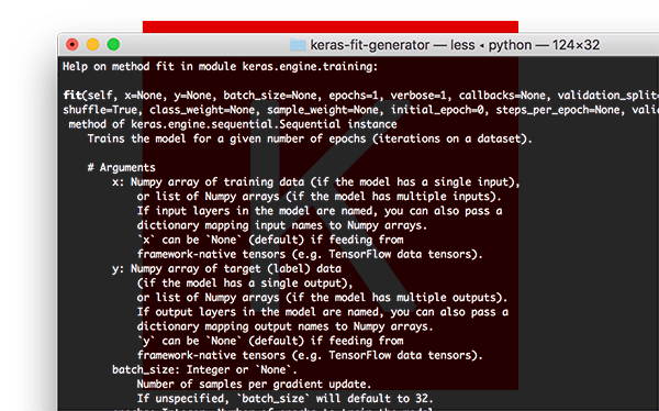
Figure 1: The Keras .fit function signature.

Let’s start with a call to

.fit

model.fit(trainX, trainY, batch_size=32, epochs=50)

Here you can see that we are supplying our training data (

trainX

trainY

We then instruct Keras to allow our model to train for

50

32

The call to

.fit

1. Our entire training set can fit into RAM
2. There is no data augmentation going on (i.e., there is no need for Keras generators)

Instead, our network will be trained on the raw data.

The raw data itself will fit into memory — we have no need to move old batches of data out of RAM and move new batches of data into RAM.

Furthermore, we will not be manipulating the training data on the fly using data augmentation.

The Keras fit_generator function

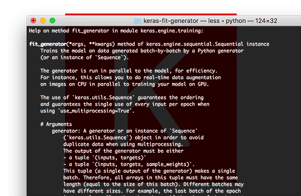
Figure 2: The Keras .fit_generator function allows for data augmentation and data generators.

For small, simplistic datasets it’s perfectly acceptable to use Keras’

.fit

These datasets are often not very challenging and do not require any data augmentation.

However, real-world datasets are rarely that simple:

• Real-world datasets are often too large to fit into memory.
• They also tend to be challenging, requiring us to perform data augmentation to avoid overfitting and increase the ability of our model to generalize.

In those situations we need to utilize Keras’

.fit_generator

# initialize the number of epochs and batch size
EPOCHS = 100
BS = 32

# construct the training image generator for data augmentation
aug = ImageDataGenerator(rotation_range=20, zoom_range=0.15,
	width_shift_range=0.2, height_shift_range=0.2, shear_range=0.15,
	horizontal_flip=True, fill_mode="nearest")

# train the network
H = model.fit_generator(aug.flow(trainX, trainY, batch_size=BS),
	validation_data=(testX, testY), steps_per_epoch=len(trainX) // BS,
	epochs=EPOCHS)

Here we start by first initializing the number of epochs we are going to train our network for along with the batch size.

We then initialize

aug

ImageDataGenerator

Performing data augmentation is a form of regularization, enabling our model to generalize better.

However, applying data augmentation implies that our training data is no longer “static” — the data is constantly changing.

Each new batch of data is randomly adjusted according to the parameters supplied to

ImageDataGenerator

Thus, we now need to utilize Keras’

.fit_generator

As the name suggests, the

.fit_generator

The function itself is a Python generator.

Internally, Keras is using the following process when training a model with

.fit_generator

1. Keras calls the generator function supplied to

   .fit_generator

     (in this case,

   aug.flow

    ).
2. The generator function yields a batch of size

   BS

     to the

   .fit_generator

     function.
3. The

   .fit_generator

     function accepts the batch of data, performs backpropagation, and updates the weights in our model.
4. This process is repeated until we have reached the desired number of epochs.

You’ll notice we now need to supply a

steps_per_epoch

.fit_generator

.fit

Why do we need

steps_per_epoch

Keep in mind that a Keras data generator is meant to loop infinitely — it should never return or exit.

Since the function is intended to loop infinitely, Keras has no ability to determine when one epoch starts and a new epoch begins.

Therefore, we compute the

steps_per_epoch

The Keras train_on_batch function

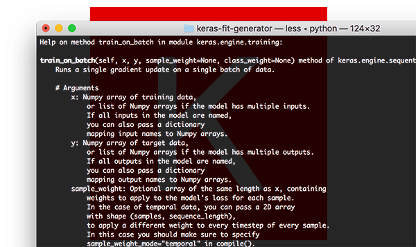
Figure 3: The .train_on_batch function in Keras offers expert-level control over training Keras models.

For deep learning practitioners looking for the finest-grained control over training your Keras models, you may wish to use the

.train_on_batch

model.train_on_batch(batchX, batchY)

The

train_on_batch

The batch of data can be of arbitrary size (i.e., it does not require an explicit batch size to be provided).

The data itself can be generated however you like as well. This data could be raw images on disk or data that has been modified or augmented in some manner.

You’ll typically use the

.train_on_batch

If you find yourself asking if you need the

.train_on_batch

In 99% of the situations you will not need such fine-grained control over training your deep learning models. Instead, a custom Keras

.fit_generator

That said, it’s good to know that the function exists if you ever need it.

I typically only recommend using the

.train_on_batch

An image dataset…as a CSV file?

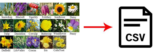
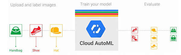
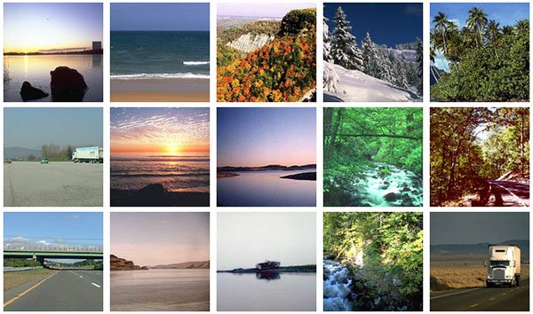
Figure 4: The Flowers-17 dataset has been serialized into two CSV files (training and evaluation). In this blog post we’ll write a custom Keras generator to parse the CSV data and yield batches of images to the .fit_generator function. (credits: image & icon)

The dataset we will be using here today is the Flowers-17 dataset, a collection of 17 different flower species with 80 images per class.

Our goal will be to train a Keras Convolutional Neural Network to correctly classify each species of flowers.

However, there’s a bit of a twist to this project:

• Instead of working with the raw image files residing on disk…
• …I’ve serialized the entire image dataset to two CSV files (one for training, and one for evaluation).

To construct each CSV file I:

• Looped over all images in our input dataset
• Resized them to 64×64 pixels
• Flattened the 64x64x3=12,288 RGB pixel intensities into a single list
• Wrote 12,288 pixel values + class label to the CSV file (one per line)

Our goal is to now write a custom Keras generator to parse the CSV file and yield batches of images and labels to the

.fit_generator

Wait, why bother with a CSV file if you already have the images?

Today’s tutorial is meant to be an example of how to implement your own Keras generator for the

.fit_generator

In the real-world datasets are not nicely curated for you:

• You may have unstructured directories of images.
• You could be working with both images and text.
• Your images could be serialized in a particular format, whether that’s a CSV file, a Caffe or TensorFlow record file, etc.

In these situations, you will need to know how to write your own Keras generator functions.

Keep in mind that it’s not the particular data format that’s important here — it’s the actual process of writing your own Keras generator that you need to learn (and that’s exactly what’s covered in the rest of the tutorial).

Project structure

Let’s inspect the project tree for today’s example:

$ tree --dirsfirst
.
├── pyimagesearch
│   ├── __init__.py
│   └── minivggnet.py
├── flowers17_testing.csv
├── flowers17_training.csv
├── plot.png
└── train.py

1 directory, 6 files

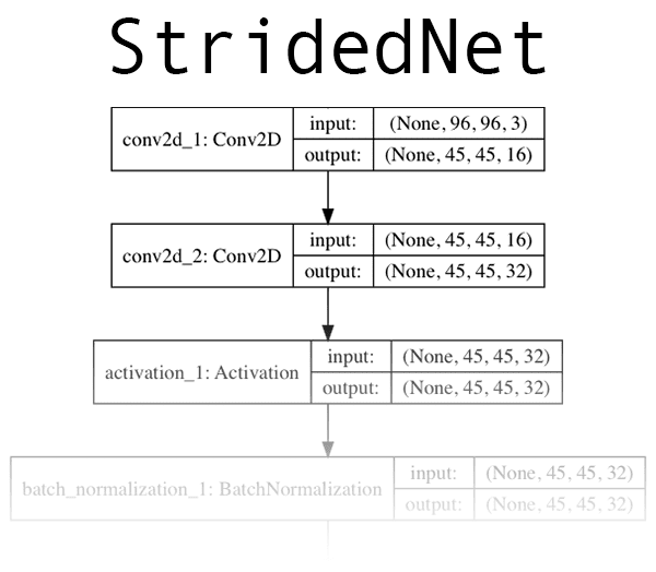
Today we’ll be using the MiniVGGNet CNN. We won’t be covering the implementation here today as I’ll assume you already know how to implement a CNN. If not, no worries — just refer to my Keras tutorial.

Our serialized image dataset is contained within

flowers17_training.csv

flowers17_testing.csv

We’ll be reviewing

train.py

Implementing a custom Keras fit_generator function

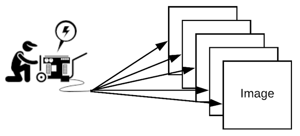
Figure 5: What’s our fuel source for our ImageDataGenerator? Two CSV files with serialized image text strings. The generator engine is the ImageDataGenerator from Keras coupled with our custom csv_image_generator. The generator will burn the CSV fuel to create batches of images for training.

Let’s go ahead and get started.

I’ll be assuming you have the following libraries installed on your system:

• NumPy
• TensorFlow + Keras
• Scikit-learn
• Matplotlib

Each of these packages can be installed via pip in your virtual environment. If you have virtualenvwrapper installed you can create an environment with

mkvirtualenv

workon

$ mkvirtualenv cv -p python3
$ workon cv
$ pip install numpy
$ pip install tensorflow # or tensorflow-gpu
$ pip install keras
$ pip install scikit-learn
$ pip install matplotlib

Once your virtual environment is set up, you can proceed with writing the training script. Make sure you use the “Downloads” section of today’s post grab the source code and Flowers-17 CSV image dataset.

Open up the

train.py

# set the matplotlib backend so figures can be saved in the background
import matplotlib
matplotlib.use("Agg")

# import the necessary packages
from keras.preprocessing.image import ImageDataGenerator
from keras.optimizers import SGD
from sklearn.preprocessing import LabelBinarizer
from sklearn.metrics import classification_report
from pyimagesearch.minivggnet import MiniVGGNet
import matplotlib.pyplot as plt
import numpy as np

Lines 2-12 import our required packages and modules. Since we’ll be saving our training plot to disk, Line 3 sets

matplotlib

Notable imports include

ImageDataGenerator

MiniVGGNet

Let’s define the

csv_image_generator

def csv_image_generator(inputPath, bs, lb, mode="train", aug=None):
	# open the CSV file for reading
	f = open(inputPath, "r")

On Line 14 we’ve defined the

csv_image_generator

.fit_generator

As such, the function accepts the following parameters:

• inputPath

   : the path to the CSV dataset file.

• bs

   : The batch size. We’ll be using 32.

• lb

   : A label binarizer object which contains our class labels.

• mode

   : (default is

  "train"

   ) If and only if the

  mode=="eval"

   , then a special accommodation is made to not apply data augmentation via the

  aug

    object (if one is supplied).

• aug

   : (default is

  None

   ) If an augmentation object is specified, then we’ll apply it before we yield our images and labels.

On Line 16 we’ll go ahead and open the CSV data file for reading.

Let’s begin looping over the lines of data:

# loop indefinitely
	while True:
		# initialize our batches of images and labels
		images = []
		labels = []

Each line of data in the CSV file contains an image serialized as a text string. Again, I generated the text strings from the Flowers-17 dataset. Additionally, I know this isn’t the most efficient way to store an image, but it is great for the purposes of this example.

Our Keras generator must loop indefinitely as is defined on Line 19. The

.fit_generator

csv_image_generator

And furthermore, Keras maintains a cache/queue of data, ensuring the model we are training always has data to train on. Keras constantly keeps this queue full so even if you have reached the total number of epochs to train for, keep in mind that Keras is still feeding the data generator, keeping data in the queue.

Always make sure your function returns data, otherwise, Keras will error out saying it could not obtain more training data from your generator.

At each iteration of the loop, we’ll reinitialize our

images

labels

From there, we’ll begin appending images and labels to these lists until we’ve reached our batch size:

# keep looping until we reach our batch size
		while len(images) < bs:
			# attempt to read the next line of the CSV file
			line = f.readline()

			# check to see if the line is empty, indicating we have
			# reached the end of the file
			if line == "":
				# reset the file pointer to the beginning of the file
				# and re-read the line
				f.seek(0)
				line = f.readline()

				# if we are evaluating we should now break from our
				# loop to ensure we don't continue to fill up the
				# batch from samples at the beginning of the file
				if mode == "eval":
					break

			# extract the label and construct the image
			line = line.strip().split(",")
			label = line[0]
			image = np.array([int(x) for x in line[1:]], dtype="uint8")
			image = image.reshape((64, 64, 3))

			# update our corresponding batches lists
			images.append(image)
			labels.append(label)

Let’s walk through this loop:

• First, we read a

  line

    from our text file object,

  f

    (Line 27).
• If

  line

    is empty:
  • …we reset our file pointer and try to read a

    line

      (Lines 34 and 35).
  • And if we’re in evaluation

    mode

     , we go ahead and

    break

      from the loop (Lines 40 and 41).
• At this point, we’ll parse our

  image

    and

  label

    from the CSV file (Lines 44-46).
• We go ahead and call

  .reshape

    to reshape our 1D array into our image which is 64×64 pixels with 3 color channels (Line 47).
• Finally, we append the

  image

    and

  label

    to their respective lists, repeating this process until our batch of images is full (Lines 50 and 51).

Note: The key to making evaluation work here is that we supply the number of

steps

model.predict_generator

With our batch of images and corresponding labels ready, we can now take two steps before yielding our batch:

# one-hot encode the labels
		labels = lb.transform(np.array(labels))

		# if the data augmentation object is not None, apply it
		if aug is not None:
			(images, labels) = next(aug.flow(np.array(images),
				labels, batch_size=bs))

		# yield the batch to the calling function
		yield (np.array(images), labels)

Our final steps include:

• One-hot encoding

  labels

    (Line 54)
• Applying data augmentation if necessary (Lines 57-59)

Finally, our generator “yields” our array of images and our list of labels to the calling function on request (Line 62). If you aren’t familiar with the

yield

Let’s initialize our training parameters:

# initialize the paths to our training and testing CSV files
TRAIN_CSV = "flowers17_training.csv"
TEST_CSV = "flowers17_testing.csv"

# initialize the number of epochs to train for and batch size
NUM_EPOCHS = 75
BS = 32

# initialize the total number of training and testing image
NUM_TRAIN_IMAGES = 0
NUM_TEST_IMAGES = 0

A number of initializations are hardcoded in this example training script:

• Our training and testing CSV filepaths (Lines 65 and 66).
• The number of epochs and batch size for training (Lines 69 and 70).
• Two variables which will hold the number of training and testing images (Lines 73 and 74).

Let’s take a look at the next block of code:

# open the training CSV file, then initialize the unique set of class
# labels in the dataset along with the testing labels
f = open(TRAIN_CSV, "r")
labels = set()
testLabels = []

# loop over all rows of the CSV file
for line in f:
	# extract the class label, update the labels list, and increment
	# the total number of training images
	label = line.strip().split(",")[0]
	labels.add(label)
	NUM_TRAIN_IMAGES += 1

# close the training CSV file and open the testing CSV file
f.close()
f = open(TEST_CSV, "r")

# loop over the lines in the testing file
for line in f:
	# extract the class label, update the test labels list, and
	# increment the total number of testing images
	label = line.strip().split(",")[0]
	testLabels.append(label)
	NUM_TEST_IMAGES += 1

# close the testing CSV file
f.close()

This block of code is long, but it has three purposes:

1. Extract all labels from our training dataset so that we can subsequently determine unique labels. Notice that

   labels

     is a

   set

     which only allows unique entries.
2. Assemble a list of

   testLabels

    .
3. Count the

   NUM_TRAIN_IMAGES

     and

   NUM_TEST_IMAGES

    .

Let’s build our

LabelBinarizer

# create the label binarizer for one-hot encoding labels, then encode
# the testing labels
lb = LabelBinarizer()
lb.fit(list(labels))
testLabels = lb.transform(testLabels)

# construct the training image generator for data augmentation
aug = ImageDataGenerator(rotation_range=20, zoom_range=0.15,
	width_shift_range=0.2, height_shift_range=0.2, shear_range=0.15,
	horizontal_flip=True, fill_mode="nearest")

Using the unique labels, we’ll

.fit

LabelBinarizer

We’ll also go ahead and transform our

testLabels

testLabels

From there, we’ll construct

aug

ImageDataGenerator

Now let’s initialize our training and testing image generators:

# initialize both the training and testing image generators
trainGen = csv_image_generator(TRAIN_CSV, BS, lb,
	mode="train", aug=aug)
testGen = csv_image_generator(TEST_CSV, BS, lb,
	mode="train", aug=None)

Our

trainGen

testGen

csv_image_generator

Notice the subtle similarities and differences:

• We’re using

  mode="train"

    for both generators
• Only

  trainGen

    will perform data augmentation

Let’s initialize + compile our MiniVGGNet model with Keras and begin training:

# initialize our Keras model and compile it
model = MiniVGGNet.build(64, 64, 3, len(lb.classes_))
opt = SGD(lr=1e-2, momentum=0.9, decay=1e-2 / NUM_EPOCHS)
model.compile(loss="categorical_crossentropy", optimizer=opt,
	metrics=["accuracy"])

# train the network
print("[INFO] training w/ generator...")
H = model.fit_generator(
	trainGen,
	steps_per_epoch=NUM_TRAIN_IMAGES // BS,
	validation_data=testGen,
	validation_steps=NUM_TEST_IMAGES // BS,
	epochs=NUM_EPOCHS)

Lines 123-126 compile our model. We’re using a Stochastic Gradient Descent optimizer with a hardcoded initial learning rate of

1e-2

On Lines 130-135 we call

.fit_generator

The

trainGen

.fit_generator

Notice how we compute the steps per epoch and validation steps based on number of images and batch size. It’s paramount that we supply the

steps_per_epoch

Now let’s evaluate the results of training:

# re-initialize our testing data generator, this time for evaluating
testGen = csv_image_generator(TEST_CSV, BS, lb,
	mode="eval", aug=None)

# make predictions on the testing images, finding the index of the
# label with the corresponding largest predicted probability
predIdxs = model.predict_generator(testGen,
	steps=(NUM_TEST_IMAGES // BS) + 1)
predIdxs = np.argmax(predIdxs, axis=1)

# show a nicely formatted classification report
print("[INFO] evaluating network...")
print(classification_report(testLabels.argmax(axis=1), predIdxs,
	target_names=lb.classes_))

We go ahead and re-initialize our

testGen

mode

"eval"

After re-initialization, we make predictions using our

.predict_generator

testGen

Using the

testLabels

predIdxs

classification_report

As a final step, we’ll use our training history dictionary,

H

# plot the training loss and accuracy
N = NUM_EPOCHS
plt.style.use("ggplot")
plt.figure()
plt.plot(np.arange(0, N), H.history["loss"], label="train_loss")
plt.plot(np.arange(0, N), H.history["val_loss"], label="val_loss")
plt.plot(np.arange(0, N), H.history["acc"], label="train_acc")
plt.plot(np.arange(0, N), H.history["val_acc"], label="val_acc")
plt.title("Training Loss and Accuracy on Dataset")
plt.xlabel("Epoch #")
plt.ylabel("Loss/Accuracy")
plt.legend(loc="lower left")
plt.savefig("plot.png")

The accuracy/loss plot is generated and saved to disk as

plot.png

Training a Keras model using fit_generator and evaluating with predict_generator

To train our Keras model using our custom data generator, make sure you use the “Downloads” section to download the source code and example CSV image dataset.

From there, open a terminal, navigate to where you downloaded the source code + dataset, and execute the following command:

$ python train.py
Using TensorFlow backend.
[INFO] training w/ generator...
Epoch 1/75
31/31 [==============================] - 5s - loss: 3.5171 - acc: 0.1381 - val_loss: 14.5745 - val_acc: 0.0906
Epoch 2/75
31/31 [==============================] - 4s - loss: 3.0275 - acc: 0.2258 - val_loss: 14.1294 - val_acc: 0.1187
Epoch 3/75
31/31 [==============================] - 4s - loss: 2.6691 - acc: 0.2823 - val_loss: 14.4892 - val_acc: 0.0781
...
Epoch 73/75
31/31 [==============================] - 4s - loss: 0.3604 - acc: 0.8720 - val_loss: 0.7640 - val_acc: 0.7656
Epoch 74/75
31/31 [==============================] - 4s - loss: 0.3185 - acc: 0.8851 - val_loss: 0.7459 - val_acc: 0.7812
Epoch 75/75
31/31 [==============================] - 4s - loss: 0.3346 - acc: 0.8821 - val_loss: 0.8337 - val_acc: 0.7719
[INFO] evaluating network...
             precision    recall  f1-score   support

   bluebell       0.95      0.86      0.90        21
  buttercup       0.50      0.93      0.65        15
  coltsfoot       0.71      0.71      0.71        21
    cowslip       0.71      0.75      0.73        20
     crocus       0.78      0.58      0.67        24
   daffodil       0.81      0.63      0.71        27
      daisy       0.93      0.78      0.85        18
  dandelion       0.71      0.94      0.81        18
 fritillary       0.90      0.86      0.88        22
       iris       1.00      0.79      0.88        24
 lilyvalley       0.80      0.73      0.76        22
      pansy       0.83      0.83      0.83        18
   snowdrop       0.71      0.68      0.70        22
  sunflower       1.00      0.94      0.97        18
  tigerlily       1.00      0.93      0.96        14
      tulip       0.50      0.31      0.38        16
 windflower       0.59      1.00      0.74        20

avg / total       0.80      0.77      0.77       340

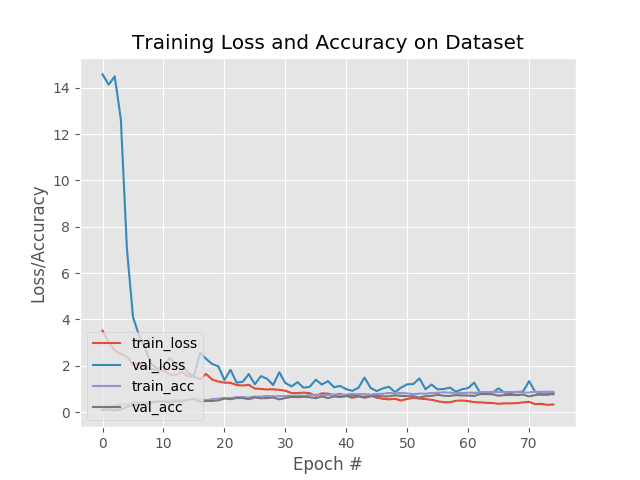
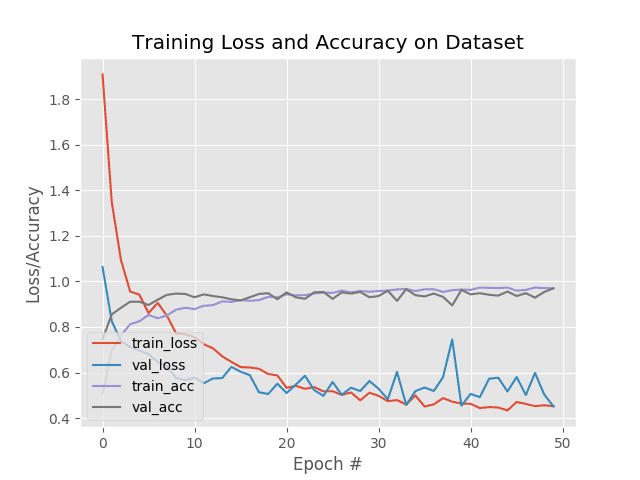
Figure 6: Our accuracy/loss Keras training plot for MiniVGGNet trained on Flowers-17.

Here you can see that our network has obtained 80% accuracy on the evaluation set, which is quite respectable for the relatively shallow CNN used.

Most importantly, you learned how to utilize:

• Data generators

• .fit_generator

• .predict_generator

…all to train and evaluate your own custom Keras model!

Again, it’s not the actual format of the data itself that’s important here. Instead of CSV files, we could have been working with Caffe or TensorFlow record files, a combination of numerical/categorical data along with images, or any other synthesis of data that you may encounter in the real-world.

Instead, it’s the actual process of implementing your own Keras data generator that matters here.

Follow the steps in this tutorial and you’ll have a blueprint that you can use for implementing your own Keras data generators.

Need more hands-on experience working with large datasets and Keras generators?

Figure 7: My deep learning book, Deep Learning for Computer with Python.

Are you interested in gaining more hands-on experience working with large datasets and deep learning?

If so, you’ll want to take a look at my book, Deep Learning for Computer Vision with Python.

Inside the book you’ll find:

1. Super practical walkthroughs that present solutions to actual, real-world image classification problems on large datasets.
2. Hands-on tutorials (with lots of code) that not only show you the algorithms behind deep learning for computer vision but their implementations as well, including how to work with large amounts of data and train Keras deep learning models on top of your dataset.
3. A no-nonsense teaching style that is guaranteed help you master deep learning for image understanding and visual recognition.

To learn more about my deep learning book (and grab your free PDF of sample chapters and table of contents), just click here.

Summary

In this tutorial you learned the differences between Keras’ three primary functions used to train a deep neural network:

1. .fit

    : Used when the entire training dataset can fit into memory and no data augmentation is applied.

2. .fit_generator

    : Should be used when either (1) the dataset is too large to fit into memory, (2) data augmentation needs to be applied, or (3) in any situation when it’s more convenient to yield training data in batches (i.e., using the

   flow_from_directory

     function).

3. .train_on_batch

    : Can be used to train a Keras model on a single batch of data. Should be utilized only when you need the finest-grained control training your network, such as in situations where your data iterator is highly complex.

From there, we discovered how to:

1. Implement our own custom Keras generator function
2. Use our custom generator along with Keras’

   .fit_generator

     to train our deep neural network

You can use today’s example code as a template when implementing your own Keras generators in your own projects.

I hope you enjoyed today’s blog post!

To download the source code to this post, and be notified when future tutorials are published here on PyImageSearch, just enter your email address in the form below!

Downloads:

If you would like to download the code and images used in this post, please enter your email address in the form below. Not only will you get a .zip of the code, I’ll also send you a FREE 17-page Resource Guide on Computer Vision, OpenCV, and Deep Learning. Inside you'll find my hand-picked tutorials, books, courses, and libraries to help you master CV and DL! Sound good? If so, enter your email address and I’ll send you the code immediately!

Email address:

The post How to use Keras fit and fit_generator (a hands-on tutorial) appeared first on PyImageSearch.

In today’s tutorial, we are going to discuss the Keras Conv2D class, including the most important parameters you need to tune when training your own Convolutional Neural Networks (CNNs). From there we are going to use the Keras Conv2D class to implement a simple CNN. We’ll then train and evaluate this CNN on the CALTECH-101 dataset.

The inspiration for today’s post came from PyImageSearch reader, Danny.

Danny asked:

Hi Adrian, I’m having some trouble understanding the parameters to Keras’ Conv2D class.

Which ones are the important ones?

Which ones should I just leave at their default values?

I’m a bit new to deep learning so I’m a bit confused on how to choose the parameter values when creating my own CNN.

Danny asks a great question — there are quite a few parameters to Keras’ Conv2D class. The sheer number can be a bit overwhelming if you’re new to the world of computer vision and deep learning.

In today’s tutorial I’m going to discuss each of the parameters to the Keras Conv2D class, explain each one, and provide examples of situations where and when you would want to set specific values, enabling you to:

1. Quickly determine if you need to utilize a specific parameter to the Keras Conv2D class
2. Decide on a proper value for that specific parameter
3. Effectively train your own Convolutional Neural Network

Overall, my goal is to help reduce any confusion, anxiety, or frustration when using Keras’ Conv2D class. After going through this tutorial you will have a strong understanding of the Keras Conv2D parameters.

To learn more about the Keras Conv2D class and convolutional layers, just keep reading!

Keras Conv2D and Convolutional Layers

In the first part of this tutorial, we are going to discuss the parameters to the Keras Conv2D class.

From there we are going to utilize the Conv2D class to implement a simple Convolutional Neural Network.

We’ll then take our CNN implementation and then train it on the CALTECH-101 dataset.

Finally, we’ll evaluate the network and examine its performance.

Let’s go ahead and get started!

The Keras Conv2D class

The Keras Conv2D class constructor has the following signature:

keras.layers.Conv2D(filters, kernel_size, strides=(1, 1),
  padding='valid', data_format=None, dilation_rate=(1, 1),
  activation=None, use_bias=True, kernel_initializer='glorot_uniform',
  bias_initializer='zeros', kernel_regularizer=None,
  bias_regularizer=None, activity_regularizer=None,
  kernel_constraint=None, bias_constraint=None)

Looks a bit overwhelming, right?

How in the world are you supposed to properly set these values?

No worries — let’s examine each of these parameters individually, giving you a strong understanding of not only what each parameter controls but also how to properly set each parameter as well.

filters

Figure 1: The Keras Conv2D parameter, filters determines the number of kernels to convolve with the input volume. Each of these operations produces a 2D activation map.

The first required Conv2D parameter is the number of

filters

Layers early in the network architecture (i.e., closer to the actual input image) learn fewer convolutional filters while layers deeper in the network (i.e., closer to the output predictions) will learn more filters.

Conv2D layers in between will learn more filters than the early Conv2D layers but fewer filters than the layers closer to the output. Let’s go ahead and take a look at an example:

model.add(Conv2D(32, (3, 3), padding="same", activation="relu"))
model.add(MaxPooling2D(pool_size=(2, 2)))
...
model.add(Conv2D(64, (3, 3), padding="same", activation="relu"))
model.add(MaxPooling2D(pool_size=(2, 2)))
...
model.add(Conv2D(128, (3, 3), padding="same", activation="relu"))
model.add(MaxPooling2D(pool_size=(2, 2)))
...
model.add(Activation("softmax"))

On Line 1 we learn a total of

32

We then learn

64

The final Conv2D layer learns

128

Notice at as our output spatial volume is decreasing our number of filters learned is increasing — this is a common practice in designing CNN architectures and one I recommend you do as well. As far as choosing the appropriate number of

filters

You may need to tune the exact value depending on (1) the complexity of your dataset and (2) the depth of your neural network, but I recommend starting with filters in the range [32, 64, 128] in the earlier and increasing up to [256, 512, 1024] in the deeper layers.

Again, the exact range of the values may be different for you, but start with a smaller number of filters and only increase when necessary.

kernel_size

Figure 2: The Keras deep learning Conv2D parameter, filter_size, determines the dimensions of the kernel. Common dimensions include 1×1, 3×3, 5×5, and 7×7 which can be passed as (1, 1), (3, 3), (5, 5), or (7, 7) tuples.

The second required parameter you need to provide to the Keras Conv2D class is the

kernel_size

The

kernel_size

Typical values for

kernel_size

(1, 1)

(3, 3)

(5, 5)

(7, 7)

So, when do you use each?

If your input images are greater than 128×128 you may choose to use a kernel size > 3 to help (1) learn larger spatial filters and (2) to help reduce volume size.

Other networks, such as VGGNet, exclusively use

(3, 3)

More advanced architectures such as Inception, ResNet, and SqueezeNet design entire micro-architectures which are “modules” inside the network that learn local features at different scales (i.e., 1×1, 3×3, and 5×5) and then combine the outputs.

A great example can be seen in the Inception module below:

Figure 3: The Inception/GoogLeNet CNN architecture uses “micro-architecture” modules inside the network that learn local features at different scales (filter_size) and then combine the outputs.

The Residual module in the ResNet architecture uses 1×1 and 3×3 filters as a form of dimensionality reduction which helps to keep the number of parameters in the network low (or as low as possible given the depth of the network):

Figure 4: The ResNet “Residual module” uses 1×1 and 3×3 filters for dimensionality reduction. This helps keep the overall network smaller with fewer parameters.

So, how should you choose your

filter_size

First, examine your input image — is it larger than 128×128?

If so, consider using a 5×5 or 7×7 kernel to learn larger features and then quickly reduce spatial dimensions — then start working with 3×3 kernels:

model.add(Conv2D(32, (7, 7), activation="relu"))
...
model.add(Conv2D(32, (3, 3), activation="relu"))

If your images are smaller than 128×128 you may want to consider sticking with strictly 1×1 and 3×3 filters.

And if you intend on using ResNet or Inception-like modules you’ll want to implement the associated modules and architectures by hand. Covering how to implement these modules is outside the scope of this tutorial, but if you’re interested in learning more about them (including how to hand-code them), please refer to my book, Deep Learning for Computer Vision with Python.

strides

The

strides

The

strides

(1, 1)

1. A given convolutional filter is applied to the current location of the input volume
2. The filter takes a 1-pixel step to the right and again the filter is applied to the input volume
3. This process is performed until we reach the far-right border of the volume in which we move our filter one pixel down and then start again from the far left

Typically you’ll leave the

strides

(1, 1)

(2, 2)

Typically you’ll see strides of 2×2 as a replacement to max pooling:

model.add(Conv2D(128, (3, 3), strides=(1, 1), activation="relu"))
model.add(Conv2D(128, (3, 3), strides=(1, 1), activation="relu"))
model.add(Conv2D(128, (3, 3), strides=(2, 2), activation="relu"))

Here we can see our first two Conv2D layers have a stride of 1×1. The final Conv2D layer; however, takes the place of a max pooling layer, and instead reduces the spatial dimensions of the output volume via strided convolution.

In 2014, Springenber et al. published a paper entitled Striving for Simplicity: The All Convolutional Net which demonstrated that replacing pooling layers with strided convolutions can increase accuracy in some situations.

ResNet, a popular CNN, has embraced this finding — if you ever look at the source code to a ResNet implementation (or implement it yourself), you’ll see that ResNet replies on strided convolution rather than max pooling to reduce spatial dimensions in between residual modules.

padding

Figure 5: A 3×3 kernel applied to an image with padding. The Keras Conv2D padding parameter accepts either "valid" (no padding) or "same" (padding + preserving spatial dimensions). This animation was contributed to StackOverflow (source).

The

padding

valid

same

With the

valid

The following example would naturally reduce the spatial dimensions of our volume:

model.add(Conv2D(32, (3, 3), padding="valid"))

Note: See this tutorial on the basics of convolution if you need help understanding how and why spatial dimensions naturally reduce when applying convolutions.

If you instead want to preserve the spatial dimensions of the volume such that the output volume size matches the input volume size, then you would want to supply a value of

same

padding

model.add(Conv2D(32, (3, 3), padding="same"))

While the default Keras Conv2D value is

valid

same

1. Max pooling
2. Strided convolution

I would recommend that you use a similar approach to padding with the Keras Conv2D class as well.

data_format

Figure 6: Keras, as a high-level framework, supports multiple deep learning backends. Thus, it includes support for both “channels last” and “channels first” channel ordering.

The data format value in the Conv2D class can be either

channels_last

channels_first

• The TensorFlow backend to Keras uses channels last ordering.
• The Theano backend uses channels first ordering.

You typically shouldn’t have to ever touch this value as Keras for two reasons:

1. You are more than likely using the TensorFlow backend to Keras
2. And if not, you’ve likely already updated your

   ~/.keras/keras.json

     configuration file to set your backend and associated channel ordering

My advice is to never explicitly set the

data_format

dilation_rate

Figure 7: The Keras deep learning Conv2D parameter, dilation_rate, accepts a 2-tuple of integers to control dilated convolution (source).

The

dilation_rate

You may use dilated convolution when:

1. You are working with higher resolution images but fine-grained details are still important
2. You are constructing a network with fewer parameters

Discussing dilated convolution is outside the scope of this tutorial so if you are interested in learning more, please refer to this tutorial.

activation

Figure 8: Keras provides a number of common activation functions. The activation parameter to Conv2D is a matter of convenience and allows the activation function for use after convolution to be specified.

The

activation

In the following example we perform convolution and then apply a ReLU activation function:

model.add(Conv2D(32, (3, 3), activation="relu"))

The above code is equivalent to:

model.add(Conv2D(32, (3, 3)))
model.add(Activation("relu"))

My advice?

Use the

activation

use_bias

The

use_bias

Typically you’ll want to leave this value as

True

I recommend keep the bias unless you have a good reason not to.

kernel_initializer and bias_initializer

Figure 9: Keras offers a number of initializers for the Conv2D class. Initializers can be used to help train deeper neural networks more effectively.

The

kernel_initializer

Similarly, the

bias_initializer

A full list of initializers can be found in the Keras documentation; however, here is what I recommend:

1. Leave the

   bias_initialization

     alone — it will by default filled with zeros (you’ll rarely if ever, have to change the bias initialization method.
2. The

   kernel_initializer

     defaults to

   glorot_uniform

    , the Xavier Glorot uniform initialization method, which is perfectly fine for the majority of tasks; however, for deeper neural networks you may want to use 

   he_normal

     (MSRA/He et al. initialization) which works especially well when your network has a large number of parameters (i.e., VGGNet).

In the vast majority of CNNs I implement I am either using

glorot_uniform

he_normal

kernel_regularizer, bias_regularizer, and activity_regularizer

Figure 10: Regularization hyperparameters should be adjusted especially when working with large datasets and really deep networks. The kernel_regularizer parameter in particular is one that I adjust often to reduce overfitting and increase the ability for a model to generalize to unfamiliar images.

The

kernel_regularizer

bias_regularizer

activity_regularizer

Applying regularization helps you to:

1. Reduce the effects of overfitting
2. Increase the ability of your model to generalize

When working with large datasets and deep neural networks applying regularization is typically a must.

Normally you’ll encounter either L1 or L2 regularization being applied — I will use L2 regularization on my networks if I detect signs of overfitting:

from keras.regularizers import l2
...
model.add(Conv2D(32, (3, 3), activation="relu"),
	kernel_regularizer=l2(0.0005))

The amount of regularization you apply is a hyperparameter you will need to tune for your own dataset, but I find values of 0.0001-0.001 are good ranges to start with.

I would suggest leaving your bias regularizer alone — regularizing the bias typically has very little impact on reducing overfitting.

I also suggest leaving the

activity_regularizer

While weight regularization methods operate on weights themselves, f(W), where f is the activation function and W are the weights, an activity regularizer instead operates on the outputs, f(O), where O is the outputs of a layer.

Unless there is a very specific reason you’re looking to regularize the output it’s best to leave this parameter alone.

kernel_constraint and bias_constraint

The final two parameters to the Keras Conv2D class are the

kernel_constraint

bias_constraint

These parameters allow you to impose constraints on the Conv2D layer, including non-negativity, unit normalization, and min-max normalization.

You can see the full list of supported constraints in the Keras documentation.

Again, I would recommend leaving both the kernel constraint and bias constraint alone unless you have a specific reason to impose constraints on the Conv2D layer.

The CALTECH-101 (subset) dataset

Figure 11: The CALTECH-101 dataset consists of 101 object categories with 40-80 images per class. The dataset for today’s blog post example consists of just 4 of those classes: faces, leopards, motorbikes, and airplanes (source).

The CALTECH-101 dataset is a dataset of 101 object categories with 40 to 800 images per class.

Most images have approximately 50 images per class.

The goal of the dataset is to train a model capable of predicting the target class.

Prior to the resurgence of neural networks and deep learning, the state-of-the-art accuracy on was only ~65%.

However, by using Convolutional Neural Networks, it’s been possible to achieve 90%+ accuracy (as He et al. demonstrated in their 2014 paper, Spatial Pyramid Pooling in Deep Convolutional Networks for Visual Recognition).

Today we are going to implement a simple yet effective CNN that is capable of achieving 96%+ accuracy, on a 4-class subset of the dataset:

• Faces: 436 images
• Leopards: 201 images
• Motorbikes: 799 images
• Airplanes: 801 images

The reason we are using a subset of the dataset is so you can easily follow along with this example and train the network from scratch, even if you do not have a GPU.

Again, the purpose of this tutorial is not meant to deliver state-of-the-art results on CALTECH-101 — it’s instead meant to teach you the fundamentals of how to use Keras’ Conv2D class to implement and train a custom Convolutional Neural Network.

Downloading the dataset and source code

Interested in following along with today’s tutorial? If so, you’ll need to download both:

1. The source code to this post (using the “Downloads” section of the post)
2. The CALTECH-101 dataset

To download the source code to this post you can use this link. ***Adrian: Please add link***

After you have downloaded the .zip of the source code, unarchive it, and then change directory into the

keras-conv2d-example

$ cd /path/to/keras-conv2d-example

From there, use the following

wget

$ wget http://www.vision.caltech.edu/Image_Datasets/Caltech101/101_ObjectCategories.tar.gz
$ tar -zxvf 101_ObjectCategories.tar.gz

Now that we’ve downloaded our code and dataset we can move on inspecting the project structure.

Project structure

To see how our project is organized, simply use the

tree

$ tree --dirsfirst -L 2 -v
.
├── 101_ObjectCategories
...
│   ├── Faces [436 entries]
...
│   ├── Leopards [201 entries]
│   ├── Motorbikes [799 entries]
...
│   ├── airplanes [801 entries]
...
├── pyimagesearch
│   ├── __init__.py
│   └── stridednet.py
├── 101_ObjectCategories.tar.gz
├── train.py
└── plot.png

104 directories, 5 files

The first directory,

101_ObjectCategories/

The

pyimagesearch/

stridendet.py

In addition to

stridednet.py

train.py

The training script will produce a training history plot,

plot.png

A Keras Conv2D Example

Figure 12: A deep learning CNN dubbed “StridedNet” serves as the example for today’s blog post about Keras Conv2D parameters. Click to expand.

Now that we’re reviewed both (1) how the Keras Conv2D class works and (2) the dataset we’ll be training our network on, let’s go ahead and implement the Convolutional Neural Neural network we’ll be training.

The CNN we’ll be using today, “StridedNet”, is one I made up for the purposes of this tutorial.

StridedNet has three important characteristics:

1. It uses strided convolutions rather than pooling operations to reduce volume size
2. The first CONV layer uses 7×7 filters but all other layers in the network use 3×3 filters (similar to VGG)
3. The MSRA/He et al. normal distribution algorithm is used to initialize all weights in the network

Let’s go ahead and implemented StridedNet now.

Open up a new file, name it

stridednet.py

# import the necessary packages
from keras.models import Sequential
from keras.layers.normalization import BatchNormalization
from keras.layers.convolutional import Conv2D
from keras.layers.core import Activation
from keras.layers.core import Flatten
from keras.layers.core import Dropout
from keras.layers.core import Dense
from keras import backend as K

class StridedNet:
	@staticmethod
	def build(width, height, depth, classes, reg, init="he_normal"):
		# initialize the model along with the input shape to be
		# "channels last" and the channels dimension itself
		model = Sequential()
		inputShape = (height, width, depth)
		chanDim = -1

		# if we are using "channels first", update the input shape
		# and channels dimension
		if K.image_data_format() == "channels_first":
			inputShape = (depth, height, width)
			chanDim = 1

All of our Keras modules are imported on Lines 2-9, namely

Conv2D

Our

StridedNet

build

The

build

• width

   : Image width in pixels.

• height

   : The image height in pixels.

• depth

   : The number of channels for the image.

• classes

   : The number of classes the model needs to predict.

• reg

   : Regularization method.

• init

   : The kernel initializer.

The

width

height

depth

For

"channels_last"

depth

We can use the Keras backend to check the

image_data_format

"channels_first"

Let’s take a lot at how we can build the first three CONV layers:

# our first CONV layer will learn a total of 16 filters, each
		# Of which are 7x7 -- we'll then apply 2x2 strides to reduce
		# the spatial dimensions of the volume
		model.add(Conv2D(16, (7, 7), strides=(2, 2), padding="valid",
			kernel_initializer=init, kernel_regularizer=reg,
			input_shape=inputShape))

		# here we stack two CONV layers on top of each other where
		# each layerswill learn a total of 32 (3x3) filters
		model.add(Conv2D(32, (3, 3), padding="same",
			kernel_initializer=init, kernel_regularizer=reg))
		model.add(Activation("relu"))
		model.add(BatchNormalization(axis=chanDim))
		model.add(Conv2D(32, (3, 3), strides=(2, 2), padding="same",
			kernel_initializer=init, kernel_regularizer=reg))
		model.add(Activation("relu"))
		model.add(BatchNormalization(axis=chanDim))
		model.add(Dropout(0.25))

Each

Conv2D

model.add

Notice that for the first

Conv2D

inputShape

model.add

Taking into account the parameters to

Conv2D

ReLU activation is applied (refer to Figure 8) along with batch normalization and dropout.

I nearly always recommend batch normalization because it tends to stabilize training and make tuning hyperparameters easier. That said, it can double or triple your training time. Use it wisely.

Dropout’s purpose is to help your network generalize and not overfit. Neurons from the current layer, with probability p, will randomly disconnect from neurons in the next layer so that the network has to rely on the existing connections. I highly recommend utilizing dropout.

Let’s take a look at more layers of StridedNet:

# stack two more CONV layers, keeping the size of each filter
		# as 3x3 but increasing to 64 total learned filters
		model.add(Conv2D(64, (3, 3), padding="same",
			kernel_initializer=init, kernel_regularizer=reg))
		model.add(Activation("relu"))
		model.add(BatchNormalization(axis=chanDim))
		model.add(Conv2D(64, (3, 3), strides=(2, 2), padding="same",
			kernel_initializer=init, kernel_regularizer=reg))
		model.add(Activation("relu"))
		model.add(BatchNormalization(axis=chanDim))
		model.add(Dropout(0.25))

		# increase the number of filters again, this time to 128
		model.add(Conv2D(128, (3, 3), padding="same",
			kernel_initializer=init, kernel_regularizer=reg))
		model.add(Activation("relu"))
		model.add(BatchNormalization(axis=chanDim))
		model.add(Conv2D(128, (3, 3), strides=(2, 2), padding="same",
			kernel_initializer=init, kernel_regularizer=reg))
		model.add(Activation("relu"))
		model.add(BatchNormalization(axis=chanDim))
		model.add(Dropout(0.25))

The deeper the network goes, the more filters we learn.

At the end of most networks we add a fully connected layer:

# fully-connected layer
		model.add(Flatten())
		model.add(Dense(512, kernel_initializer=init))
		model.add(Activation("relu"))
		model.add(BatchNormalization())
		model.add(Dropout(0.5))

		# softmax classifier
		model.add(Dense(classes))
		model.add(Activation("softmax"))

		# return the constructed network architecture
		return model

A single fully connected layer with

512

Finally, a

"softmax"

That’s a wrap.

As you can see, Keras syntax is quite straightforward once you know what the parameters mean (

Conv2D

Let’s learn how to write a script to train StridedNet with some data!

Implementing the training script

Now that we have implemented our CNN architecture, let’s create the driver script used to train the network.

Open up the

train.py

# set the matplotlib backend so figures can be saved in the background
import matplotlib
matplotlib.use("Agg")

# import the necessary packages
from pyimagesearch.stridednet import StridedNet
from sklearn.preprocessing import LabelBinarizer
from sklearn.model_selection import train_test_split
from sklearn.metrics import classification_report
from keras.preprocessing.image import ImageDataGenerator
from keras.optimizers import Adam
from keras.regularizers import l2
from imutils import paths
import matplotlib.pyplot as plt
import numpy as np
import argparse
import cv2
import os

We import our modules and packages on Lines 2-18. Notice that we aren’t importing

Conv2D

stridednet.py

StridedNet

Our

matplotlib

We import functionality from

sklearn

• LabelBinarizer

   : For “one-hot” encoding our class labels.

• train_test_split

   : For splitting our data such that we have training and evaluation sets.

• classification_report

   : We’ll use this to print statistics from evaluation.

From

keras

• ImageDataGenerator

   : For data augmentation. See last week’s blog post for more information on Keras data generators.

• Adam

   : An optimizer alternative to SGD.

• l2

   : The regularizer we’ll be using. Scroll up to read about regularizers. Applying regularization reduces overfitting and helps with generalization.

My imutils

paths

We’ll use

argparse

cv2

Let’s go ahead and parse the command line arguments now:

# construct the argument parser and parse the arguments
ap = argparse.ArgumentParser()
ap.add_argument("-d", "--dataset", required=True,
	help="path to input dataset")
ap.add_argument("-e", "--epochs", type=int, default=50,
	help="# of epochs to train our network for")
ap.add_argument("-p", "--plot", type=str, default="plot.png",
	help="path to output loss/accuracy plot")
args = vars(ap.parse_args())

Our script can accept three command line arguments:

• --dataset

   : The path to the input dataset.

• --epochs

   : The number of epochs to train for. By

  default

   , we’ll train for

  50

    epochs.

• --plot

   : Our loss/accuracy plot will be output to disk. This argument contains the file path. By default, it is simply

  "plot.png"

   .

Let’s prepare to load our dataset:

# initialize the set of labels from the CALTECH-101 dataset we are
# going to train our network on
LABELS = set(["Faces", "Leopards", "Motorbikes", "airplanes"])

# grab the list of images in our dataset directory, then initialize
# the list of data (i.e., images) and class images
print("[INFO] loading images...")
imagePaths = list(paths.list_images(args["dataset"]))
data = []
labels = []

Before we actually load our dataset, we’ll go ahead and initialize:

• LABELS

   : The labels we’ll use for training.

• imagePaths

   : A list of image paths for the dataset directory. We’ll filter these based on the parsed class labels from the file paths soon.

• data

   : A list to hold our images that our network will be trained on.

• labels

   : A list to hold our class labels that correspond to the data.

Let’s populate our

data

labels

# loop over the image paths
for imagePath in imagePaths:
	# extract the class label from the filename
	label = imagePath.split(os.path.sep)[-2]

	# if the label of the current image is not part of of the labels
	# are interested in, then ignore the image
	if label not in LABELS:
		continue

	# load the image and resize it to be a fixed 96x96 pixels,
	# ignoring aspect ratio
	image = cv2.imread(imagePath)
	image = cv2.resize(image, (96, 96))

	# update the data and labels lists, respectively
	data.append(image)
	labels.append(label)

Beginning on Line 42, we’ll loop over all

imagePaths

• Extract the

  label

    from the path (Line 44).
• Filter only the classes in the

  LABELS

    set (Lines 48 and 49). These two lines cause us to skip any

  label

    not belonging to Faces, Leopards, Motorbikes, or Airplanes classes, respectively, as is defined on Line 32.
• Load and

  resize

    our

  image

    (Lines 53 and 54).
• And finally, add the

  image

    and

  label

    to their respective lists (Lines 57 and 58).

There are four actions taking place in the next block:

# convert the data into a NumPy array, then preprocess it by scaling
# all pixel intensities to the range [0, 1]
data = np.array(data, dtype="float") / 255.0

# perform one-hot encoding on the labels
lb = LabelBinarizer()
labels = lb.fit_transform(labels)

# partition the data into training and testing splits using 75% of
# the data for training and the remaining 25% for testing
(trainX, testX, trainY, testY) = train_test_split(data, labels,
	test_size=0.25, stratify=labels, random_state=42)

# construct the training image generator for data augmentation
aug = ImageDataGenerator(rotation_range=20, zoom_range=0.15,
	width_shift_range=0.2, height_shift_range=0.2, shear_range=0.15,
	horizontal_flip=True, fill_mode="nearest")

These actions include:

• Converting

  data

    to a NumPy array with each

  image

    scaled to the range [0, 1] (Line 62).
• Binarize our

  labels

    into “one-hot encoding” with our

  LabelBinarizer

    (Lines 65 and 66). This means that our

  labels

    are now represented numerically where “one-hot” examples might be:

  • [0, 0, 0, 1]

      for “airplane”

  • [0, 1, 0, 0]

      for “Leopards”
  • etc.
• Split our

  data

    into training and testing (Lines 70 and 71).
• Initialize our

  ImageDataGenerator

    for data augmentation (Lines 74-76). You can read more about it here.

Now we’re ready to write code to actually train our model:

# initialize the optimizer and model
print("[INFO] compiling model...")
opt = Adam(lr=1e-4, decay=1e-4 / args["epochs"])
model = StridedNet.build(width=96, height=96, depth=3,
	classes=len(lb.classes_), reg=l2(0.0005))
model.compile(loss="categorical_crossentropy", optimizer=opt,
	metrics=["accuracy"])

# train the network
print("[INFO] training network for {} epochs...".format(
	args["epochs"]))
H = model.fit_generator(aug.flow(trainX, trainY, batch_size=32),
	validation_data=(testX, testY), steps_per_epoch=len(trainX) // 32,
	epochs=args["epochs"])

Lines 80-84 prepare our

StridedNet

model

Adam

l2

From there, on Lines 89-91 we’ll fit our model to the data.  In this case, “fit” means “train” and

.fit_generator

To evaluate our model, we’ll use the

testX

classification_report

# evaluate the network
print("[INFO] evaluating network...")
predictions = model.predict(testX, batch_size=32)
print(classification_report(testY.argmax(axis=1),
	predictions.argmax(axis=1), target_names=lb.classes_))

And finally we’ll plot our accuracy/loss training history and save it to disk:

# plot the training loss and accuracy
N = args["epochs"]
plt.style.use("ggplot")
plt.figure()
plt.plot(np.arange(0, N), H.history["loss"], label="train_loss")
plt.plot(np.arange(0, N), H.history["val_loss"], label="val_loss")
plt.plot(np.arange(0, N), H.history["acc"], label="train_acc")
plt.plot(np.arange(0, N), H.history["val_acc"], label="val_acc")
plt.title("Training Loss and Accuracy on Dataset")
plt.xlabel("Epoch #")
plt.ylabel("Loss/Accuracy")
plt.legend(loc="lower left")
plt.savefig(args["plot"])

Training and evaluating our Keras CNN

At this point, we are ready to train our network!

Make sure you have used the “Downloads” section of today’s tutorial to download the source code and example images.

From there, open up a terminal, change directory to where you have downloaded the code and CALTECH-101 dataset, and then execute the following command:

$ python train.py --dataset 101_ObjectCategories
[INFO] loading images...
[INFO] compiling model...
[INFO] training network for 50 epochs...
Epoch 1/50
52/52 [==============================] - 4s 84ms/step - loss: 1.9081 - acc: 0.5060 - val_loss: 1.0628 - val_acc: 0.7460
Epoch 2/50
52/52 [==============================] - 3s 63ms/step - loss: 1.3809 - acc: 0.6925 - val_loss: 0.8254 - val_acc: 0.8551
Epoch 3/50
52/52 [==============================] - 3s 63ms/step - loss: 1.0881 - acc: 0.7637 - val_loss: 0.7368 - val_acc: 0.8837
...
Epoch 48/50
52/52 [==============================] - 3s 61ms/step - loss: 0.4525 - acc: 0.9730 - val_loss: 0.5981 - val_acc: 0.9284
Epoch 49/50
52/52 [==============================] - 3s 62ms/step - loss: 0.4582 - acc: 0.9692 - val_loss: 0.5032 - val_acc: 0.9535
Epoch 50/50
52/52 [==============================] - 3s 63ms/step - loss: 0.4511 - acc: 0.9699 - val_loss: 0.4511 - val_acc: 0.9696
[INFO] evaluating network...
              precision    recall  f1-score   support

       Faces       0.99      0.99      0.99       109
    Leopards       1.00      0.78      0.88        50
  Motorbikes       0.99      0.98      0.99       200
   airplanes       0.93      0.99      0.96       200

   micro avg       0.97      0.97      0.97       559
   macro avg       0.98      0.94      0.95       559
weighted avg       0.97      0.97      0.97       559

Figure 13: My accuracy/loss plot generated with Keras and matplotlib for training StridedNet, an example CNN to showcase Keras Conv2D parameters.

As you can see, our network is obtaining ~97% accuracy on the testing set with minimal overfitting!

You can apply deep learning to your own projects

Figure 14: My deep learning book, Deep Learning for Computer Vision with Python, is trusted by members of major universities and corporations — it has helped them and it will help you too.

You don’t need a degree in computer science or mathematics to study deep learning.

Instead, what you need is a book that is designed with the practitioner in mind — a book that not only teaches you the theory of how and why deep learning algorithms work, but then takes that theory and implements it in code so you fully understand it.

Sound too good to be true?

It’s not.

Inside my book, Deep Learning for Computer Vision with Python, you’ll find over 900+ pages of the most complete, comprehensive computer vision and deep learning education available online.

Regardless of whether you’re just getting started in deep learning or you’re already a seasoned deep learning practitioner, my book will help you master computer vision and deep learning through:

• Super practical walkthroughs that present solutions to actual, real-world problems through image classification (ResNet, Inception, etc.), object detection (Faster R-CNN, SSDs, RetinaNet), and instance segmentation (Mask R-CNNs).
• Hands-on tutorials (with lots of code) that not only show you the algorithms behind deep learning for computer vision but their implementations as well.
• A no-nonsense teaching style that is guaranteed to help you master deep learning for image understanding and visual recognition.

But don’t take my word for it — Deep Learning for Computer Vision with Python is trusted by members of major universities and corporations. It has helped them on their journey to CV/DL mastery and I have no doubt it will help you too.

To learn more (and grab your free table of contents + sample chapters PDF), just use the link below:

Summary

In today’s tutorial, we discussed convolutional layers and the Keras Conv2D class.

You now know:

• What the most important parameters are to the Keras Conv2D class (

  filters

   ,

  kernel_size

   ,

  strides

   ,

  padding

   )
• What proper values are for these parameters
• How to use the Keras Conv2D class to create your own Convolutional Neural Network
• How to train your CNN and evaluate it on an example dataset

I hope you found this tutorial helpful in understanding the parameters to Keras’ Conv2D Class — if you did, please leave a comment in the comments section.

If you would like to download the source code to this blog post (and to be notified when future tutorials are published here on PyImageSearch), just enter your email address in the form below.

Downloads:

If you would like to download the code and images used in this post, please enter your email address in the form below. Not only will you get a .zip of the code, I’ll also send you a FREE 17-page Resource Guide on Computer Vision, OpenCV, and Deep Learning. Inside you'll find my hand-picked tutorials, books, courses, and libraries to help you master CV and DL! Sound good? If so, enter your email address and I’ll send you the code immediately!

Email address:

The post Keras Conv2D and Convolutional Layers appeared first on PyImageSearch.

In this tutorial, you will learn how to use Auto-Keras, an open source alternative to Google’s AutoML, for automated machine learning and deep learning.

When training a neural network on a dataset there are two primary objectives a deep learning practitioner is trying to optimize and balance:

1. Defining a neural network architecture that lends itself to the nature of the dataset
2. Tuning a set of hyperparameters over many experiments that will lead to a model with high accuracy and ability to generalize to data outside the training and testing sets. Typical hyperparameters that need to be tuned include the optimizer algorithm (SGD, Adam, etc.), learning rate and learning rate scheduling, and regularization, to name a few

Depending on the dataset and problem, it can take a deep learning expert upwards of tens to hundreds of experiments to find a balance between neural network architecture and hyperparameters.

These experiments can add up to hundreds to thousands of hours in GPU compute time.

And that’s just for experts — what about non-deep learning experts?

Enter Auto-Keras and AutoML:

The end goal of both Auto-Keras and AutoML is to reduce the barrier to entry to performing machine learning and deep learning through the use of automated Neural Architecture Search (NAS) algorithms.

Auto-Keras and AutoML enable non-deep learning experts to train their own models with minimal domain knowledge of either deep learning or their actual data.

Using AutoML and Auto-Keras, a programmer with minimal machine learning expertise can apply these algorithms to achieve state-of-the-art performance with very little effort.

Sound too good to be true?

Well, maybe — but you’ll need to read the rest of the post first to find out why.

To learn more about AutoML (and how to automatically train and tune a neural network with Auto-Keras), just keep reading!

Auto-Keras and AutoML: A Getting Started Guide

In the first part of this blog post, we’ll discuss Automated Machine Learning (AutoML) and Neural Architecture Search (NAS), the algorithm that makes AutoML possible when applied to neural networks and deep learning.

We’ll also briefly discuss Google’s AutoML, a suite of tools and libraries allowing programmers with limited machine learning expertise to train high accuracy models on their own data.

Of course, Google’s AutoML is a proprietary algorithm (it’s a bit on the expensive side of as well).

An alternative to AutoML is the open source Auto-Keras, built around Keras and PyTorch.

I’ll then show you how to automatically train a network using Auto-Keras as well as to evaluate it.

What is Automated Machine Learning (AutoML)?

Figure 1: Auto-Keras is an alternative to Google’s AutoML. These software projects can help you train models automatically with little intervention. They are great options for novice deep learning practitioners or to obtain a baseline to beat later on.

Outside of unsupervised learning (automatically learning patterns from unlabeled data), automated machine learning for non-experts is considered the “holy grail” of machine learning.

Imagine the ability to automatically create a machine learning model via:

1. Installing a library/using a web interface
2. Pointing the library/interface to your data
3. Automatically training a model on the data without having to tune the parameters/requiring an intimate understanding of the algorithms powering it

Some companies are trying to create such solutions — a big one is Google’s AutoML.

Google AutoML enables developers and engineers with very limited machine learning experience to automatically train neural networks on their own datasets.

Under the hood Google’s AutoML algorithms are iterative:

1. Training a network on a training set
2. Evaluating the network on a testing set
3. Modifying the neural network architecture
4. Tuning hyperparameters
5. Repeating the process

The programmer or engineer using AutoML doesn’t need to define their own neural network architecture or tune the hyperparameters — AutoML is doing that for them automatically.

Neural Architecture Search (NAS) makes AutoML possible

Figure 2: Neural Architecture Search (NAS) produced a model summarized by these graphs when searching for the best CNN architecture for CIFAR-10 (source: Figure 4 of Zoph et al.)

Both Google’s AutoML and Auto-Keras are powered by an algorithm called Neural Architecture Search (NAS).

Given your input dataset, a Neural Architecture Search algorithm will automatically search for the most optimal architecture and corresponding parameters.

Neural Architecture Search essentially replaces the deep learning engineer/practitioner with a set of algorithms that automatically tunes the model!

In the context of computer vision and image recognition, a Neural Architecture Search algorithm will:

1. Accept an input training dataset
2. Optimize and find architectural building blocks called “cells” — these cells are automatically learned and may look similar to inception, residual, or squeeze/fire micro-architectures
3. Continually train and search the “NAS search space” for more optimized cells

If the user of the AutoML system is an experienced deep learning practitioner then they may decide to:

1. Run the NAS on a significantly smaller subset of the training dataset
2. Find an optimal set of architectural building blocks/cells
3. Take these cells and manually define a deeper version of the network found during the architecture search
4. Train the network on the full training set using their own expertise and best practices

Such an approach is a hybrid between a fully automated machine learning solution and one that requires an expert deep learning practitioner — often this approach will lead to better accuracy than what the NAS finds on its own.

I would recommend reading Neural Architecture Search with Reinforcement Learning (Zoph and Le, 2016) along with Learning Transferable Architectures for Scalable Image Recognition (Zoph et al., 2017) for more details on how these algorithms work.

Auto-Keras: An open source alternative to Google’s AutoML

Figure 3: The Auto-Keras package was developed by the DATA Lab team at Texas A&M University. Auto-Keras is an open source alternative to Google’s AutoML.

The Auto-Keras package, developed by the DATA Lab team at Texas A&M University, is an alternative to Google’s AutoML.

Auto-Keras also utilizes the Neural Architecture Search but applies “network morphism” (keeping network functionality while changing the architecture) along with Bayesian optimization to guide the network morphism for more efficient neural network search.

You can find the full details of the Auto-Keras framework in Jin et al.’s 2018 publication, Auto-Keras: Efficient Neural Architecture Search with Network Morphism.

Project structure

Go ahead and grab the zip from the “Downloads” section of today’s blog post.

From there you should unzip the file and navigate into it using your terminal.

Let’s inspect today’s project with the

tree

$ tree --dirsfirst
.
├── output
│   ├── 14400.txt
│   ├── 28800.txt
│   ├── 3600.txt
│   ├── 43200.txt
│   ├── 7200.txt
│   └── 86400.txt
└── train_auto_keras.py

1 directory, 7 files

Today we’re going to be reviewing a single Python script:

train_auto_keras.py

Since there will be a lot of output printed to the screen, I’ve opted to save our classification reports (generated with the help of scikit-learn’s

classification_report

output/

cat output/14400.txt

Installing Auto-Keras

Figure 4: The Auto-Keras package depends upon Python 3.6, TensorFlow, and Keras.

As the Auto-Keras GitHub repository states, Auto-Keras is in a “pre-release” state — it is not an official release.

Secondly, Auto-Keras requires Python 3.6 and is only compatible with Python 3.6.

If you are using any other version of Python other than 3.6 you will not be able to utilize the Auto-Keras package.

To check your Python version just use the following command:

$ python --version

Provided you have Python 3.6 you can install Auto-Keras using pip:

$ pip install tensorflow # or tensorflow-gpu
$ pip install keras
$ pip install autokeras

If you have any issues installing or utilizing Auto-Keras make sure you post on the official Auto-Keras GitHub Issues page where the authors will be able to help you.

Implementing our training script with Auto-Keras

Let’s go ahead and implement our training script using Auto-Keras. Open up the

train_auto_keras.py

# import the necessary packages
from sklearn.metrics import classification_report
from keras.datasets import cifar10
import autokeras as ak
import os

def main():
	# initialize the output directory
	OUTPUT_PATH = "output"

To begin, we import necessary packages on Lines 2-5:

• As previously mentioned, we’ll be using scikit-learn’s

  classification_report

    to calculate statistics which we’ll save in our output files.
• We’re going to use the CIFAR-10 Dataset, conveniently built into

  keras.datasets

   .
• Then comes our most notable import,

  autokeras

   , which I’ve imported as 

  ak

    for shorthand.
• The

  os

    module is required as we’ll accommodate path separators on various operating systems when building output file paths.

Let’s define the

main

main

Our base

OUTPUT_PATH

Now let’s initialize a list of training times for Auto-Keras:

# initialize the list of training times that we'll allow
	# Auto-Keras to train for
	TRAINING_TIMES = [
		60 * 60,		# 1 hour
		60 * 60 * 2,	# 2 hours
		60 * 60 * 4,	# 4 hours
		60 * 60 * 8,	# 8 hours
		60 * 60 * 12,	# 12 hours
		60 * 60 * 24,	# 24 hours
	]

Lines 13-20 define a set of

TRAINING_TIMES 

[1, 2, 4, 8, 12, 24]

Let’s load the CIFAR-10 dataset and initialize class names:

# load the training and testing data, then scale it into the
	# range [0, 1]
	print("[INFO] loading CIFAR-10 data...")
	((trainX, trainY), (testX, testY)) = cifar10.load_data()
	trainX = trainX.astype("float") / 255.0
	testX = testX.astype("float") / 255.0

	# initialize the label names for the CIFAR-10 dataset
	labelNames = ["airplane", "automobile", "bird", "cat", "deer",
		"dog", "frog", "horse", "ship", "truck"]

Our CIFAR-10 data is loaded and stored into training/testing splits on Line 25.

Subsequently, we’ll scale this data to the range of [0, 1] (Lines 26 and 27).

Our class

labelNames

And now let’s begin looping over our

TRAINING_TIMES

# loop over the number of seconds to allow the current Auto-Keras
	# model to train for
	for seconds in TRAINING_TIMES:
		# train our Auto-Keras model
		print("[INFO] training model for {} seconds max...".format(
			seconds))
		model = ak.ImageClassifier(verbose=True)
		model.fit(trainX, trainY, time_limit=seconds)
		model.final_fit(trainX, trainY, testX, testY, retrain=True)

		# evaluate the Auto-Keras model
		score = model.evaluate(testX, testY)
		predictions = model.predict(testX)
		report = classification_report(testY, predictions,
			target_names=labelNames)

		# write the report to disk
		p = os.path.sep.join(OUTPUT_PATH, "{}.txt".format(seconds))
		f = open(p, "w")
		f.write(report)
		f.write("\nscore: {}".format(score))
		f.close()

The code block above is the heart of today’s script. On Line 35 we’ve defined a loop over each of our

TRAINING_TIMES

• Initialize our

  model

    (

  ak.ImageClassifier

   ) and allow training to start (Lines 39 and 40). Notice that we didn’t instantiate an object for a particular CNN class as we have in previous tutorials such as this one. Nor do we need to tune hyperparameters as we typically do. Auto-Keras handles all of this for us and provides a report of its findings.
• Once the time limit has been reached, take the best

  model

    and parameters Auto-Keras has found + re-train the model (Line 41).
• Evaluate and construct the classification

  report

    (Lines 44-47).
• Write the classification

  report

    along with the accuracy

  score

    to disk so we can evaluate the effect of longer training times (Lines 50-54).

We’ll repeat this process for each of our

TRAINING_TIMES

Finally, we’ll check for and start the

main

# if this is the main thread of execution then start the process (our
# code must be wrapped like this to avoid threading issues with
# TensorFlow)
if __name__ == "__main__":
	main()

Here we’ve checked to ensure that this is the

main

main

Just 60 lines later, we’re done writing our Auto-Keras with CIFAR-10 example script. But we’re not done yet…

Training a neural network with Auto-Keras

Let’s go ahead and train our neural network using Auto-Keras.

Make sure you use the “Downloads” section of this tutorial to download the source code.

From there, open up a terminal, navigate to where you downloaded the source code, and execute the following command:

$ python train_auto_keras.py
[INFO] training model for 3600 seconds max...   
Preprocessing the images.
Preprocessing finished.

Initializing search.
Initialization finished.


+----------------------------------------------+
|               Training model 0               |
+----------------------------------------------+
Using TensorFlow backend.

No loss decrease after 5 epochs.


Saving model.
+--------------------------------------------------------------------------+
|        Model ID        |          Loss          |      Metric Value      |
+--------------------------------------------------------------------------+
|           0            |   4.816269397735596    |         0.5852         |
+--------------------------------------------------------------------------+


+----------------------------------------------+
|               Training model 1               |
+----------------------------------------------+
Using TensorFlow backend.
Epoch-14, Current Metric - 0.83:  28%|██████▊                 | 110/387 [01:02<02:46,  1.67 batch/s]Time is out.
[INFO] training model for 86400 seconds max...  
Preprocessing the images.
Preprocessing finished.

Initializing search.
Initialization finished.


+----------------------------------------------+
|               Training model 0               |
+----------------------------------------------+
Using TensorFlow backend.

No loss decrease after 5 epochs.
...
+----------------------------------------------+
|              Training model 21               |
+----------------------------------------------+
Using TensorFlow backend.

No loss decrease after 5 epochs.


+--------------------------------------------------------------------------+
|    Father Model ID     |                 Added Operation                 |
+--------------------------------------------------------------------------+
|                        |             to_deeper_model 16 ReLU             |
|           16           |               to_wider_model 16 64              |
+--------------------------------------------------------------------------+

Saving model.
+--------------------------------------------------------------------------+
|        Model ID        |          Loss          |      Metric Value      |
+--------------------------------------------------------------------------+
|           21           |   0.8843476831912994   |   0.9316000000000001   |
+--------------------------------------------------------------------------+


+----------------------------------------------+
|              Training model 22               |
+----------------------------------------------+
Using TensorFlow backend.
Epoch-3, Current Metric - 0.9:  80%|████████████████████▊     | 310/387 [03:50<00:58,  1.31 batch/s]Time is out.

No loss decrease after 30 epochs.

Here you can see that our script is instructing Auto-Keras to perform six sets of experiments.

The total training time, including the time limits + the time to re-fit the model, was a little over 3 days on an NVIDIA K80 GPU.

Auto-Keras results

Figure 5: Using Auto-Keras usually is a very time-consuming process. Training with Auto-Keras produces the best models for CIFAR-10 in the 8-12 hour range. Past that, Auto-Keras is not able to optimize further.

In Figure 5 above you can see the effect of the amount of training time (x-axis) on overall accuracy (y-axis) using Auto-Keras.

Lower training times, namely 1 and 2 hours, lead to ~73% accuracy. Once we train for 4 hours we are able to achieve up to 93% accuracy.

The best accuracy we obtain is in the 8-12 range where we achieve 95% accuracy.

Training for longer than 8-12 hours does not increase our accuracy, implying that we have reached a saturation point and Auto-Keras is not able to optimize further.

Are Auto-Keras and AutoML worth it?

Figure 6: Is Auto-Keras (or AutoML) worth it? It is certainly a great step forward in the industry and is especially helpful for those without deep learning domain knowledge. That said, seasoned deep learning experts can craft architectures + train them in significantly less time + achieve equal or greater accuracy.

Outside of unsupervised learning (automatically learning patterns from unlabeled data), automated machine learning for non-experts is considered the “holy grail” of machine learning.

Both Google’s AutoML and the open source Auto-Keras package attempt to bring machine learning to the masses, even without significant technical experience.

While Auto-Keras worked reasonably well for CIFAR-10, I ran a second set of experiments using my previous post on deep learning, medical imagery, and malaria detection.

In that previous post, I obtained 97.1% accuracy using a simplified ResNet architecture which took under one hour to train.

I then let Auto-Keras run for 24 hours on the same dataset — the result was barely 96% accuracy, less than my hand-defined architecture.

Both Google’s AutoML and Auto-Keras are great steps forward; however, automated machine learning is nowhere near solved.

Automatic machine learning (currently) does not beat having expertise in deep learning — domain expertise, specifically in the data you are working with, is absolutely critical to obtain a higher accuracy model.

My suggestion is to invest in your own knowledge, don’t rely on automated algorithms.

To be a successful deep learning practitioner and engineer you need to bring the right tool to the job. Use AutoML and Auto-Keras for what they are, tools, and then continue to fill your own toolbox with additional knowledge.

Summary

In today’s blog post, we discussed Auto-Keras and AutoML, a set of tools and libraries to perform automated machine learning and deep learning.

The end goal of both Auto-Keras and AutoML is to reduce the barrier to entry to performing machine learning and deep learning through the use of Neural Architecture Search (NAS) algorithms.

NAS algorithms, the backbone of Auto-Keras and AutoML, will automatically:

1. Define and optimize a neural network architecture
2. Tune the hyperparameters to the model

The primary benefits include:

• Being able to perform machine learning and deep learning with little expertise
• Obtaining a high accuracy model with the ability to generalize to data outside the training and testing set
• Getting up and running quickly with either a GUI interface or a simple API
• A potentially state-of-the-art performance with little effort

Of course, there is a price to be paid — two prices in fact.

First, Google’s AutoML is expensive, approximately $20/hour.

To save funds you could go with Auto-Keras, an open source alternative to Google’s AutoML, but you still need to pay for GPU compute time.

Replacing an actual deep learning expert with a NAS algorithm will require many hours of computing to search for optimal parameters.

While we achieved a high accuracy model for CIFAR-10 (~96% accuracy), when I applied Auto-Keras to my previous post on medical deep learning and malaria prediction, Auto-Keras only achieved 96.1% accuracy, a full percentage point lower than my 97% accuracy (and Auto-Keras required 2,300% more compute time!)

While Auto-Keras and AutoML may be a step in the right direction in terms of automated machine learning and deep learning, there is still quite a bit of work to be done in this area.

There is no silver bullet for solving machine learning/deep learning with off-the-shelf algorithms. Instead, I recommend you invest in yourself as a deep learning practitioner and engineer.

The skills you learn today and tomorrow will pay off tremendously in the future.

I hope you enjoyed today’s tutorial!

To download the source code to this post (and be notified when future tutorials are published here on PyImageSearch), just enter your email address in the form below!

Downloads:

If you would like to download the code and images used in this post, please enter your email address in the form below. Not only will you get a .zip of the code, I’ll also send you a FREE 17-page Resource Guide on Computer Vision, OpenCV, and Deep Learning. Inside you'll find my hand-picked tutorials, books, courses, and libraries to help you master CV and DL! Sound good? If so, enter your email address and I’ll send you the code immediately!

Email address:

The post Auto-Keras and AutoML: A Getting Started Guide appeared first on PyImageSearch.

Struggling to get started with machine learning using Python? In this step-by-step, hands-on tutorial you will learn how to perform machine learning using Python on numerical data and image data.

By the time you are finished reading this post, you will be able to get your start in machine learning.

To launch your machine learning in Python education, just keep reading!

Machine Learning in Python

Inside this tutorial, you will learn how to perform machine learning in Python on numerical data and image data.

You will learn how to operate popular Python machine learning and deep learning libraries, including two of my favorites:

• scikit-learn
• Keras

Specifically, you will learn how to:

1. Examine your problem
2. Prepare your data (raw data, feature extraction, feature engineering, etc.)
3. Spot-check a set of algorithms
4. Examine your results
5. Double-down on the algorithms that worked best

Using this technique you will be able to get your start with machine learning and Python!

Along the way, you’ll discover popular machine learning algorithms that you can use in your own projects as well, including:

1. k-Nearest Neighbors (k-NN)
2. Naïve Bayes
3. Logistic Regression
4. Support Vector Machines (SVMs)
5. Decision Trees
6. Random Forests
7. Perceptrons
8. Multi-layer, feedforward neural networks
9. Convolutional Neural Networks (CNNs)

This hands-on experience will give you the knowledge (and confidence) you need to apply machine learning in Python to your own projects.

Install the required Python machine learning libraries

Before we can get started with this tutorial you first need to make sure your system is configured for machine learning. Today’s code requires the following libraries:

• NumPy: For numerical processing with Python.
• PIL: A simple image processing library. OpenCV is not a requirement today!
• scikit-learn: Contains the machine learning algorithms we’ll cover today (we’ll need version 0.20+ which is why you see the

  --upgrade

    flag below).
• Keras and TensorFlow: For deep learning. The CPU version of TensorFlow is fine for today’s example.
• imutils: My personal package of image processing/computer vision convenience functions

Each of these can be installed in your environment (virtual environments recommended) with pip:

$ pip install numpy
$ pip install pillow
$ pip install --upgrade scikit-learn
$ pip install tensorflow # or tensorflow-gpu
$ pip install keras
$ pip install --upgrade imutils

Datasets

In order to help you gain experience performing machine learning in Python, we’ll be working with two separate datasets.

The first one, the Iris dataset, is the machine learning practitioner’s equivalent of “Hello, World!” (likely one of the first pieces of software you wrote when learning how to program).

The second dataset, 3-scenes, is an example image dataset I put together — this dataset will help you gain experience working with image data, and most importantly, learn what techniques work best for numerical/categorical datasets vs. image datasets.

Let’s go ahead and get a more intimate look at these datasets.

The Iris dataset

Figure 1: The Iris dataset is a numerical dataset describing Iris flowers. It captures measurements of their sepal and petal length/width. Using these measurements we can attempt to predict flower species with Python and machine learning. (source)

The Iris dataset is arguably one of the most simplistic machine learning datasets — it is often used to help teach programmers and engineers the fundamentals of machine learning and pattern recognition.

We call this dataset the “Iris dataset” because it captures attributes of three Iris flower species:

1. Iris Setosa
2. Iris Versicolor
3. Iris Virginica

Each species of flower is quantified via four numerical attributes, all measured in centimeters:

1. Sepal length
2. Sepal width
3. Petal length
4. Petal width

Our goal is to train a machine learning model to correctly predict the flower species from the measured attributes.

It’s important to note that one of the classes is linearly separable from the other two — the latter are not linearly separable from each other.

In order to correctly classify these the flower species, we will need a non-linear model.

It’s extremely common to need a non-linear model when performing machine learning with Python in the real world — the rest of this tutorial will help you gain this experience and be more prepared to conduct machine learning on your own datasets.

The 3-scenes image dataset

Figure 2: The 3-scenes dataset consists of pictures of coastlines, forests, and highways. We’ll use Python to train machine learning and deep learning models.

The second dataset we’ll be using to train machine learning models is called the 3-scenes dataset and includes 948 total images of 3 scenes:

• Coast (360 of images)
• Forest (328 of images)
• Highway (260 of images)

The 3-scenes dataset was created by sampling the 8-scenes dataset from Oliva and Torralba’s 2001 paper, Modeling the shape of the scene: a holistic representation of the spatial envelope.

Our goal will be to train machine learning and deep learning models with Python to correctly recognize each of these scenes.

I have included the 3-scenes dataset in the “Downloads” section of this tutorial. Make sure you download the dataset + code to this blog post before continuing.

Steps to perform machine learning in Python

Figure 3: Creating a machine learning model with Python is a process that should be approached systematically with an engineering mindset. These five steps are repeatable and will yield quality machine learning and deep learning models.

Whenever you perform machine learning in Python I recommend starting with a simple 5-step process:

1. Examine your problem
2. Prepare your data (raw data, feature extraction, feature engineering, etc.)
3. Spot-check a set of algorithms
4. Examine your results
5. Double-down on the algorithms that worked best

This pipeline will evolve as your machine learning experience grows, but for beginners, this is the machine learning process I recommend for getting started.

To start, we must examine the problem.

Ask yourself:

• What type of data am I working with? Numerical? Categorical? Images?
• What is the end goal of my model?
• How will I define and measure “accuracy”?
• Given my current knowledge of machine learning, do I know any algorithms that work well on these types of problems?

The last question, in particular, is critical — the more you apply machine learning in Python, the more experience you will gain.

Based on your previous experience you may already know an algorithm that works well.

From there, you need to prepare your data.

Typically this step involves loading your data from disk, examining it, and deciding if you need to perform feature extraction or feature engineering.

Feature extraction is the process of applying an algorithm to quantify your data in some manner.

For example, when working with images we may wish to compute histograms to summarize the distribution of pixel intensities in the image — in this manner, we can characterize the color of the image.

Feature engineering, on the other hand, is the process of transforming your raw input data into a representation that better represents the underlying problem.

Feature engineering is a more advanced technique and one I recommend you explore once you already have some experience with machine learning and Python.

Next, you’ll want to spot-check a set of algorithms.

What do I mean by spot-checking?

Simply take a set of machine learning algorithms and apply them to the dataset!

You’ll likely want to stuff the following machine learning algorithms in your toolbox:

1. A linear model (ex. Logistic Regression, Linear SVM),
2. A few non-linear models (ex. RBF SVMs, SGD classifiers),
3. Some tree and ensemble-based models (ex. Decision Trees, Random Forests).
4. A few neural networks, if applicable (Multi-layer Perceptrons, Convolutional Neural Networks)

Try to bring a robust set of machine learning models to the problem — your goal here is to gain experience on your problem/project by identifying which machine learning algorithms performed well on the problem and which ones did not.

Once you’ve defined your set of models, train them and evaluate the results.

Which machine learning models worked well? Which models performed poorly?

Take your results and use them to double-down your efforts on the machine learning models that performed while discarding the ones that didn’t.

Over time you will start to see patterns emerge across multiple experiments and projects.

You’ll start to develop a “sixth sense” of what machine learning algorithms perform well and in what situation.

For example, you may discover that Random Forests work very well when applied to projects that have many real-valued features.

On the other hand, you might note that Logistic Regression can handle sparse, high-dimensional spaces well.

You may even find that Convolutional Neural Networks work great for image classification (which they do).

Use your knowledge here to supplement traditional machine learning education — the best way to learn machine learning with Python is to simply roll up your sleeves and get your hands dirty!

A machine learning education based on practical experience (supplemented with some super basic theory) will take you a long way on your machine learning journey!

Let’s get our hands dirty!

Now that we have discussed the fundamentals of machine learning, including the steps required to perform machine learning in Python, let’s get our hands dirty.

In the next section, we’ll briefly review our directory and project structure for this tutorial.

Note: I recommend you use the “Downloads” section of the tutorial to download the source code and example data so you can easily follow along.

Once we’ve reviewed the directory structure for the machine learning project we will implement two Python scripts:

1. The first script will be used to train machine learning algorithms on numerical data (i.e., the Iris dataset)
2. The second Python script will be utilized to train machine learning on image data (i.e., the 3-scenes dataset)

As a bonus we’ll implement two more Python scripts, each of these dedicated to neural networks and deep learning:

1. We’ll start by implementing a Python script that will train a neural network on the Iris dataset
2. Secondly, you’ll learn how to train your first Convolutional Neural Network on the 3-scenes dataset

Let’s get started by first reviewing our project structure.

Our machine learning project structure

Be sure to grab the “Downloads” associated with this blog post.

From there you can unzip the archive and inspect the contents:

$ tree --dirsfirst --filelimit 10
.
├── 3scenes
│   ├── coast [360 entries]
│   ├── forest [328 entries]
│   └── highway [260 entries]
├── classify_iris.py
├── classify_images.py
├── nn_iris.py
└── basic_cnn.py

4 directories, 4 files

The Iris dataset is built into scikit-learn. The 3-scenes dataset, however, is not. I’ve included it in the

3scenes/

We’ll be reviewing four Python machine learning scripts today:

• classify_iris.py

   : Loads the Iris dataset and can apply any one of seven machine learning algorithms with a simple command line argument switch.

• classify_images.py

   : Gathers our image dataset (3-scenes) and applies any one of seven Python machine learning algorithms

• nn_iris.py

   : Applies a simple multi-layer neural network to the Iris dataset

• basic_cnn.py

   : Builds a Convolutional Neural Network (CNN) and trains a model using the 3-scenes dataset

Implementing Python machine learning for numerical data

Figure 4: Over time, many statistical machine learning approaches have been developed. You can use this map from the scikit-learn team as a guide for the most popular methods. Expand.

The first script we are going to implement is

classify_iris.py

Once implemented, we’ll be able to use

classify_iris.py

Let’s get started — open up the

classify_iris.py

# import the necessary packages
from sklearn.neighbors import KNeighborsClassifier
from sklearn.naive_bayes import GaussianNB
from sklearn.linear_model import LogisticRegression
from sklearn.svm import SVC
from sklearn.tree import DecisionTreeClassifier
from sklearn.ensemble import RandomForestClassifier
from sklearn.neural_network import MLPClassifier
from sklearn.model_selection import train_test_split
from sklearn.metrics import classification_report
from sklearn.datasets import load_iris
import argparse

# construct the argument parser and parse the arguments
ap = argparse.ArgumentParser()
ap.add_argument("-m", "--model", type=str, default="knn",
	help="type of python machine learning model to use")
args = vars(ap.parse_args())

Lines 2-12 import our required packages, specifically:

• Our Python machine learning methods from scikit-learn (Lines 2-8)
• A dataset splitting method used to separate our data into training and testing subsets (Line 9)
• The classification report utility from scikit-learn which will print a summarization of our machine learning results (Line 10)
• Our Iris dataset, built into scikit-learn (Line 11)
• A tool for command line argument parsing called

  argparse

    (Line 12)

Using

argparse

--model

--model

# define the dictionary of models our script can use, where the key
# to the dictionary is the name of the model (supplied via command
# line argument) and the value is the model itself
models = {
	"knn": KNeighborsClassifier(n_neighbors=1),
	"naive_bayes": GaussianNB(),
	"logit": LogisticRegression(solver="lbfgs", multi_class="auto"),
	"svm": SVC(kernel="rbf", gamma="auto"),
	"decision_tree": DecisionTreeClassifier(),
	"random_forest": RandomForestClassifier(n_estimators=100),
	"mlp": MLPClassifier()
}

The

models

• k-Nearest Neighbor (k-NN)
• Naïve Bayes
• Logistic Regression
• Support Vector Machines (SVMs)
• Decision Trees
• Random Forests
• Perceptrons

The keys can be entered directly in the terminal following the

--model

$ python classify_irs.py --model knn

From there the

KNeighborClassifier

Moving on, let’s load and split our data:

# load the Iris dataset and perform a training and testing split,
# using 75% of the data for training and 25% for evaluation
print("[INFO] loading data...")
dataset = load_iris()
(trainX, testX, trainY, testY) = train_test_split(dataset.data,
	dataset.target, random_state=3, test_size=0.25)

Our dataset is easily loaded with the dedicated

load_iris

train_test_split

The final step is to train and evaluate our model:

# train the model
print("[INFO] using '{}' model".format(args["model"]))
model = models[args["model"]]
model.fit(trainX, trainY)

# make predictions on our data and show a classification report
print("[INFO] evaluating...")
predictions = model.predict(testX)
print(classification_report(testY, predictions,
	target_names=dataset.target_names))

Lines 42 and 43 train the Python machine learning

model

.fit

From there, we evaluate the

model

print

classification_report

Implementing Python machine learning for images

Figure 5: A linear classifier example for implementing Python machine learning for image classification (Inspired by Karpathy’s example in the CS231n course).

The following script,

classify_images.py

It is very similar to our previous Iris dataset classification script, so be sure to compare the two as you follow along.

Let’s implement this script now:

# import the necessary packages
from sklearn.neighbors import KNeighborsClassifier
from sklearn.naive_bayes import GaussianNB
from sklearn.linear_model import LogisticRegression
from sklearn.svm import SVC
from sklearn.tree import DecisionTreeClassifier
from sklearn.ensemble import RandomForestClassifier
from sklearn.neural_network import MLPClassifier
from sklearn.preprocessing import LabelEncoder
from sklearn.model_selection import train_test_split
from sklearn.metrics import classification_report
from PIL import Image
from imutils import paths
import numpy as np
import argparse
import os

First, we import our necessary packages on Lines 2-16. It looks like a lot, but you’ll recognize most of them from the previous script. The additional imports for this script include:

• The

  LabelEncoder

    will be used to transform textual labels into numbers (Line 9).
• A basic image processing tool called PIL/Pillow (Line 12). We’re using this in place of OpenCV today, mainly because it is easier to install.
• My handy module,

  paths

   , for easily grabbing image paths from disk (Line 13). This is included in my personal imutils package which I’ve released to GitHub and PyPi.
• NumPy will be used for numerical computations (Line 14).
• Python’s built-in

  os

    module (Line 16). We’ll use it for accommodating path separators among different operating systems.

You’ll see how each of the imports is used in the coming lines of code.

Next let’s define a function called

extract_color_stats

def extract_color_stats(image):
	# split the input image into its respective RGB color channels
	# and then create a feature vector with 6 values: the mean and
	# standard deviation for each of the 3 channels, respectively
	(R, G, B) = image.split()
	features = [np.mean(R), np.mean(G), np.mean(B), np.std(R),
		np.std(G), np.std(B)]

	# return our set of features
	return features

Most machine learning algorithms perform very poorly on raw pixel data. Instead, we perform feature extraction to characterize the contents of the images.

Here we seek to quantify the color of the image by extracting the mean and standard deviation for each color channel in the image.

Given three channels of the image (Red, Green, and Blue), along with two features for each (mean and standard deviation), we have 3 x 2 = 6 total features to quantify the image. We form a feature vector by concatenating the values.

In fact, that’s exactly what the 

extract_color_stats

• We split the three color channels from the

  image

    on Line 22.
• And then the feature vector is built on Lines 23 and 24 where you can see we’re using NumPy to calculate the mean and standard deviation for each channel

We’ll be using this function to calculate a feature vector for each image in the dataset.

Let’s go ahead and parse two command line arguments:

# construct the argument parser and parse the arguments
ap = argparse.ArgumentParser()
ap.add_argument("-d", "--dataset", type=str, default="3scenes",
	help="path to directory containing the '3scenes' dataset")
ap.add_argument("-m", "--model", type=str, default="knn",
	help="type of python machine learning model to use")
args = vars(ap.parse_args())

Where the previous script had one argument, this script has two command line arguments:

• --dataset

   : The path to the 3-scenes dataset residing on disk.

• --model

   : The Python machine learning model to employ.

Again, we have seven machine learning models to choose from with the

--model

# define the dictionary of models our script can use, where the key
# to the dictionary is the name of the model (supplied via command
# line argument) and the value is the model itself
models = {
	"knn": KNeighborsClassifier(n_neighbors=1),
	"naive_bayes": GaussianNB(),
	"logit": LogisticRegression(solver="lbfgs", multi_class="auto"),
	"svm": SVC(kernel="linear"),
	"decision_tree": DecisionTreeClassifier(),
	"random_forest": RandomForestClassifier(n_estimators=100),
	"mlp": MLPClassifier()
}

After defining the

models

# grab all image paths in the input dataset directory, initialize our
# list of extracted features and corresponding labels
print("[INFO] extracting image features...")
imagePaths = paths.list_images(args["dataset"])
data = []
labels = []

# loop over our input images
for imagePath in imagePaths:
	# load the input image from disk, compute color channel
	# statistics, and then update our data list
	image = Image.open(imagePath)
	features = extract_color_stats(image)
	data.append(features)

	# extract the class label from the file path and update the
	# labels list
	label = imagePath.split(os.path.sep)[-2]
	labels.append(label)

Our

imagePaths

I’ve defined two lists,

data

labels

data

labels

Lines 58-68 consist of a loop over the

imagePaths

1. Load each

   image

     (Line 61).
2. Extract a color stats feature vector (mean and standard deviation of each channel) from the

   image

     using the function previously defined (Line 62).
3. Then on Line 63 the feature vector is added to our

   data

     list.
4. Finally, the class

   label

     is extracted from the path and appended to the corresponding

   labels

     list (Lines 67 and 68).

Now, let’s encode our

labels

# encode the labels, converting them from strings to integers
le = LabelEncoder()
labels = le.fit_transform(labels)

# perform a training and testing split, using 75% of the data for
# training and 25% for evaluation
(trainX, testX, trainY, testY) = train_test_split(data, labels,
	test_size=0.25)

Our textual 

labels

LabelEncoder

Just as in our Iris classification script, we split our data into 75% for training and 25% for testing (Lines 76 and 77).

Finally, we can train and evaluate our model:

# train the model
print("[INFO] using '{}' model".format(args["model"]))
model = models[args["model"]]
model.fit(trainX, trainY)

# make predictions on our data and show a classification report
print("[INFO] evaluating...")
predictions = model.predict(testX)
print(classification_report(testY, predictions,
	target_names=le.classes_))

These lines are nearly identical to the Iris classification script. We’re fitting (training) our

model

classification_report

Speaking of results, now that we’re finished implementing both

classify_irs.py

classify_images.py

k-Nearest Neighbor (k-NN)

Figure 6: The k-Nearest Neighbor (k-NN) method is one of the simplest machine learning algorithms.

The k-Nearest Neighbors classifier is by far the most simple image classification algorithm.

In fact, it’s so simple that it doesn’t actually “learn” anything. Instead, this algorithm relies on the distance between feature vectors. Simply put, the k-NN algorithm classifies unknown data points by finding the most common class among the k closest examples.

Each data point in the k closest data points casts a vote and the category with the highest number of votes wins!

Or, in plain English: “Tell me who your neighbors are, and I’ll tell you who you are.”

For example, in Figure 6 above we see three sets of our flowers:

• Daises
• Pansies
• Sunflowers

We have plotted each of the flower images according to their lightness of the petals (color) and the size of the petals (this is an arbitrary example so excuse the non-formality).

We can clearly see the image the new image is a sunflower, but what does k-NN think given our new image is equal distance to one pansy and two sunflowers?

Well, k-NN would examine the three closest neighbors (k=3) and since there are two votes for sunflowers versus one vote for pansies, the sunflower class would be selected.

To put k-NN in action, make sure you’ve used the “Downloads” section of the tutorial to download the source code and example datasets.

From there, open up a terminal and execute the following command:

$ python classify_iris.py 
[INFO] loading data...
[INFO] using 'knn' model
[INFO] evaluating...
              precision    recall  f1-score   support

      setosa       1.00      1.00      1.00        15
  versicolor       0.92      0.92      0.92        12
   virginica       0.91      0.91      0.91        11

   micro avg       0.95      0.95      0.95        38
   macro avg       0.94      0.94      0.94        38

Here you can see that k-NN is obtaining 95% accuracy on the Iris dataset, not a bad start!

Let’s look at our 3-scenes dataset:

python classify_images.py --model knn
[INFO] extracting image features...
[INFO] using 'knn' model
[INFO] evaluating...
              precision    recall  f1-score   support

       coast       0.84      0.68      0.75       105
      forest       0.78      0.77      0.77        78
     highway       0.56      0.78      0.65        54

   micro avg       0.73      0.73      0.73       237
   macro avg       0.72      0.74      0.72       237
weighted avg       0.75      0.73      0.73       237

On the 3-scenes dataset, the k-NN algorithm is obtaining 75% accuracy.

In particular, k-NN is struggling to recognize the “highway” class (~56% accuracy).

We’ll be exploring methods to improve our image classification accuracy in the rest of this tutorial.

For more information on how the k-Nearest Neighbors algorithm works, be sure to refer to this post.

Naïve Bayes

Figure 7: The Naïve Bayes machine learning algorithm is based upon Bayes’ theorem (source).

After k-NN, Naïve Bayes is often the first true machine learning algorithm a practitioner will study.

The algorithm itself has been around since the 1950s and is often used to obtain baselines for future experiments (especially in domains related to text retrieval).

The Naïve Bayes algorithm is made possible due to Bayes’ theorem (Figure 7).

Essentially, Naïve Bayes formulates classification as an expected probability.

Given our input data, D, we seek to compute the probability of a given class, C.

Formally, this becomes P(C | D).

To actually compute the probability we compute the numerator of Figure 7 (ignoring the denominator).

The expression can be interpreted as:

1. Computing the probability of our input data given the class (ex., the probability of a given flower being Iris Setosa having a sepal length of 4.9cm)
2. Then multiplying by the probability of us encountering that class throughout the population of the data (ex. the probability of even encountering the Iris Setosa class in the first place)

Let’s go ahead and apply the Naïve Bayes algorithm to the Iris dataset:

$ python classify_iris.py --model naive_bayes
[INFO] loading data...
[INFO] using 'naive_bayes' model
[INFO] evaluating...
              precision    recall  f1-score   support

      setosa       1.00      1.00      1.00        15
  versicolor       1.00      0.92      0.96        12
   virginica       0.92      1.00      0.96        11

   micro avg       0.97      0.97      0.97        38
   macro avg       0.97      0.97      0.97        38
weighted avg       0.98      0.97      0.97        38

We are now up to 98% accuracy, a marked increase from the k-NN algorithm!

Now let’s apply Naïve Bayes to the 3-scenes dataset for image classification:

$ python classify_images.py --model naive_bayes
[INFO] extracting image features...
[INFO] using 'naive_bayes' model
[INFO] evaluating...
              precision    recall  f1-score   support

       coast       0.69      0.40      0.50        88
      forest       0.68      0.82      0.74        84
     highway       0.61      0.78      0.68        65

   micro avg       0.65      0.65      0.65       237
   macro avg       0.66      0.67      0.64       237
weighted avg       0.66      0.65      0.64       237

Uh oh!

It looks like we only obtained 66% accuracy here.

Does that mean that k-NN is better than Naïve Bayes and that we should always use k-NN for image classification?

Not so fast.

All we can say here is that for this particular project and for this particular set of extracted features the k-NN machine learning algorithm outperformed Naive Bayes.

We cannot say that k-NN is better than Naïve Bayes and that we should always use k-NN instead.

Thinking that one machine learning algorithm is always better than the other is a trap I see many new machine learning practitioners fall into — don’t make that mistake.

For more information on the Naïve Bayes machine learning algorithm, be sure to refer to this excellent article.

Logistic Regression

Figure 8: Logistic Regression is a machine learning algorithm based on a logistic function always in the range [0, 1]. Similar to linear regression, but based on a different function, every machine learning and Python enthusiast needs to know Logistic Regression (source).

Logistic Regression is a supervised classification algorithm often used to predict the probability of a class label (the output of a Logistic Regression algorithm is always in the range [0, 1]).

Logistic Regression is heavily used in machine learning and is an algorithm any machine learning practitioner needs Logistic Regression in their Python toolbox.

Let’s apply Logistic Regression to the Iris dataset:

$ python classify_iris.py --model logit
[INFO] loading data...
[INFO] using 'logit' model
[INFO] evaluating...
              precision    recall  f1-score   support

      setosa       1.00      1.00      1.00        15
  versicolor       1.00      0.92      0.96        12
   virginica       0.92      1.00      0.96        11

   micro avg       0.97      0.97      0.97        38
   macro avg       0.97      0.97      0.97        38
weighted avg       0.98      0.97      0.97        38

Here we are able to obtain 98% classification accuracy!

And furthermore, note that both the Setosa and Versicolor classes are classified 100% correctly!

Now let’s apply Logistic Regression to the task of image classification:

$ python classify_images.py --model logit
[INFO] extracting image features...
[INFO] using 'logit' model
[INFO] evaluating...
              precision    recall  f1-score   support

       coast       0.67      0.67      0.67        92
      forest       0.79      0.82      0.80        82
     highway       0.61      0.57      0.59        63

   micro avg       0.70      0.70      0.70       237
   macro avg       0.69      0.69      0.69       237
weighted avg       0.69      0.70      0.69       237

Logistic Regression performs slightly better than Naive Bayes here, obtaining 69% accuracy but in order to beat k-NN we’ll need a more powerful Python machine learning algorithm.

Support Vector Machines (SVMs)

Figure 9: Python machine learning practitioners will often apply Support Vector Machines (SVMs) to their problems. SVMs are based on the concept of a hyperplane and the perpendicular distance to it as shown in 2-dimensions (the hyperplane concept applies to higher dimensions as well).

Support Vector Machines (SVMs) are extremely powerful machine learning algorithms capable of learning separating hyperplanes on non-linear datasets through the kernel trick.

If a set of data points are not linearly separable in an N-dimensional space we can project them to a higher dimension — and perhaps in this higher dimensional space the data points are linearly separable.

The problem with SVMs is that it can be a pain to tune the knobs on an SVM to get it to work properly, especially for a new Python machine learning practitioner.

When using SVMs it often takes many experiments with your dataset to determine:

1. The appropriate kernel type (linear, polynomial, radial basis function, etc.)
2. Any parameters to the kernel function (ex. degree of the polynomial)

If, at first, your SVM is not obtaining reasonable accuracy you’ll want to go back and tune the kernel and associated parameters — tuning those knobs of the SVM is critical to obtaining a good machine learning model. With that said, let’s apply an SVM to our Iris dataset:

$ python classify_iris.py --model svm
[INFO] loading data...
[INFO] using 'svm' model
[INFO] evaluating...
              precision    recall  f1-score   support

      setosa       1.00      1.00      1.00        15
  versicolor       1.00      0.92      0.96        12
   virginica       0.92      1.00      0.96        11

   micro avg       0.97      0.97      0.97        38
   macro avg       0.97      0.97      0.97        38
weighted avg       0.98      0.97      0.97        38

Just like Logistic Regression, our SVM obtains 98% accuracy — in order to obtain 100% accuracy on the Iris dataset with an SVM, we would need to further tune the parameters to the kernel.

Let’s apply our SVM to the 3-scenes dataset:

$ python classify_images.py --model svm
[INFO] extracting image features...
[INFO] using 'svm' model
[INFO] evaluating...
              precision    recall  f1-score   support

       coast       0.84      0.76      0.80        92
      forest       0.86      0.93      0.89        84
     highway       0.78      0.80      0.79        61

   micro avg       0.83      0.83      0.83       237
   macro avg       0.83      0.83      0.83       237

Wow, 83% accuracy!

That’s the best accuracy we’ve seen thus far!

Clearly, when tuned properly, SVMs lend themselves well to non-linearly separable datasets.

Decision Trees

Figure 10: The concept of Decision Trees for machine learning classification can easily be explained with this figure. Given a feature vector and “set of questions” the bottom leaf represents the class. As you can see we’ll either “Go to the movies” or “Go to the beach”. There are two leaves for “Go to the movies” (nearly all complex decision trees will have multiple paths to arrive at the same conclusion with some shortcutting others).

The basic idea behind a decision tree is to break classification down into a set of choices about each entry in our feature vector.

We start at the root of the tree and then progress down to the leaves where the actual classification is made.

Unlike many machine learning algorithms such which may appear as a “black box” learning algorithm (where the route to the decision can be hard to interpret and understand), decision trees can be quite intuitive — we can actually visualize and interpret the choice the tree is making and then follow the appropriate path to classification.

For example, let’s pretend we are going to the beach for our vacation. We wake up the first morning of our vacation and check the weather report — sunny and 90 degrees Fahrenheit.

That leaves us with a decision to make: “What should we do today? Go to the beach? Or see a movie?”

Subconsciously, we may solve the problem by constructing a decision tree of our own (Figure 10).

First, we need to know if it’s sunny outside.

A quick check of the weather app on our smartphone confirms that it is indeed sunny.

We then follow the Sunny=Yes branch and arrive at the next decision — is it warmer than 70 degrees out?

Again, after checking the weather app we can confirm that it will be > 70 degrees outside today.

Following the >70=Yes branch leads us to a leaf of the tree and the final decision — it looks like we are going to the beach!

Internally, decision trees examine our input data and look for the best possible nodes/values to split on using algorithms such as CART or ID3. The tree is then automatically built for us and we are able to make predictions.

Let’s go ahead and apply the decision tree algorithm to the Iris dataset:

$ python classify_iris.py --model decision_tree
[INFO] loading data...
[INFO] using 'decision_tree' model
[INFO] evaluating...
              precision    recall  f1-score   support

      setosa       1.00      1.00      1.00        15
  versicolor       0.92      0.92      0.92        12
   virginica       0.91      0.91      0.91        11

   micro avg       0.95      0.95      0.95        38
   macro avg       0.94      0.94      0.94        38
weighted avg       0.95      0.95      0.95        38

Our decision tree is able to obtain 95% accuracy.

What about our image classification project?

$ python classify_images.py --model decision_tree
[INFO] extracting image features...
[INFO] using 'decision_tree' model
[INFO] evaluating...
              precision    recall  f1-score   support

       coast       0.71      0.74      0.72        85
      forest       0.76      0.80      0.78        83
     highway       0.77      0.68      0.72        69

   micro avg       0.74      0.74      0.74       237
   macro avg       0.75      0.74      0.74       237
weighted avg       0.74      0.74      0.74       237

Here we obtain 74% accuracy — not the best but certainly not the worst either.

Random Forests

Figure 11: A Random Forest is a collection of decision trees. This machine learning method injects a level of “randomness” into the algorithm via bootstrapping and random node splits. The final classification result is calculated by tabulation/voting. Random Forests tend to be more accurate than decision trees. (source)

Since a forest is a collection of trees, a Random Forest is a collection of decision trees.

However, as the name suggestions, Random Forests inject a level of “randomness” that is not present in decision trees — this randomness is applied at two points in the algorithm.

• Bootstrapping — Random Forest classifiers train each individual decision tree on a bootstrapped sample from the original training data. Essentially, bootstrapping is sampling with replacement a total of D times. Bootstrapping is used to improve the accuracy of our machine learning algorithms while reducing the risk of overfitting.
• Randomness in node splits — For each decision tree a Random Forest trains, the Random Forest will only give the decision tree a portion of the possible features.

In practice, injecting randomness into the Random Forest classifier by bootstrapping training samples for each tree, followed by only allowing a subset of the features to be used for each tree, typically leads to a more accurate classifier.

At prediction time, each decision tree is queried and then the meta-Random Forest algorithm tabulates the final results.

Let’s try our Random Forest on the Iris dataset:

$ python classify_iris.py --model random_forest
[INFO] loading data...
[INFO] using 'random_forest' model
[INFO] evaluating...
              precision    recall  f1-score   support

      setosa       1.00      1.00      1.00        15
  versicolor       1.00      0.83      0.91        12
   virginica       0.85      1.00      0.92        11

   micro avg       0.95      0.95      0.95        38
   macro avg       0.95      0.94      0.94        38
weighted avg       0.96      0.95      0.95        38

As we can see, our Random Forest obtains 96% accuracy, slightly better than using just a single decision tree.

But what about for image classification?

Do Random Forests work well for our 3-scenes dataset?

$ python classify_images.py --model random_forest
[INFO] extracting image features...
[INFO] using 'random_forest' model
[INFO] evaluating...
              precision    recall  f1-score   support

       coast       0.80      0.83      0.81        84
      forest       0.92      0.84      0.88        90
     highway       0.77      0.81      0.79        63

   micro avg       0.83      0.83      0.83       237
   macro avg       0.83      0.83      0.83       237
weighted avg       0.84      0.83      0.83       237

Using a Random Forest we’re able to obtain 84% accuracy, a full 10% better than using just a decision tree.

In general, if you find that decision trees work well for your machine learning and Python project, you may want to try Random Forests as well!

Neural Networks

Figure 12: Neural Networks are machine learning algorithms which are inspired by how the brains work. The Perceptron, a linear model, accepts a set of weights, computes the weighted sum, and then applies a step function to determine the class label.

One of the most common neural network models is the Perceptron, a linear model used for classification.

A Perceptron accepts a set of inputs, takes the dot product between the inputs and the weights, computes a weighted sum, and then applies a step function to determine the output class label.

We typically don’t use the original formulation of Perceptrons as we now have more advanced machine learning and deep learning models. Furthermore, since the advent of the backpropagation algorithm, we can train multi-layer Perceptrons (MLP).

Combined with non-linear activation functions, MLPs can solve non-linearly separable datasets as well.

Let’s apply a Multi-layer Perceptron machine learning algorithm to our Iris dataset using Python and scikit-learn:

$ python classify_iris.py --model mlp
[INFO] loading data...
[INFO] using 'mlp' model
[INFO] evaluating...
              precision    recall  f1-score   support

      setosa       1.00      1.00      1.00        15
  versicolor       1.00      0.92      0.96        12
   virginica       0.92      1.00      0.96        11

   micro avg       0.97      0.97      0.97        38
   macro avg       0.97      0.97      0.97        38
weighted avg       0.98      0.97      0.97        38

Our MLP performs well here, obtaining 98% classification accuracy.

Let’s move on to image classification with an MLP:

$ python classify_images.py --model mlp
[INFO] extracting image features...
[INFO] using 'mlp' model
[INFO] evaluating...
              precision    recall  f1-score   support

       coast       0.72      0.91      0.80        86
      forest       0.92      0.89      0.90        79
     highway       0.79      0.58      0.67        72

   micro avg       0.80      0.80      0.80       237
   macro avg       0.81      0.79      0.79       237
weighted avg       0.81      0.80      0.80       237

The MLP reaches 81% accuracy here — quite respectable given the simplicity of the model!

Deep Learning and Deep Neural Networks

Figure 13: Python is arguably the most popular language for Deep Learning, a subfield of machine learning. Deep Learning consists of neural networks with many hidden layers. The process of backpropagation tunes the weights iteratively as data is passed through the network. (source)

If you’re interested in machine learning and Python then you’ve likely encountered the term deep learning as well.

What exactly is deep learning?

And what makes it different than standard machine learning?

Well, to start, it’s first important to understand that deep learning is a subfield of machine learning, which is, in turn, a subfield of the larger Artificial Intelligence (AI) field.

The term “deep learning” comes from training neural networks with many hidden layers.

In fact, in the 1990s it was extremely challenging to train neural networks with more than two hidden layers due to (paraphrasing Geoff Hinton):

1. Our labeled datasets being too small
2. Our computers being far too slow
3. Not being able to properly initialize our neural network weights prior to training
4. Using the wrong type of nonlinearity function

It’s a different story now. We now have:

1. Faster computers
2. Highly optimized hardware (i.e., GPUs)
3. Large, labeled datasets
4. A better understanding of weight initialization
5. Superior activation functions

All of this has culminated at exactly the right time to give rise to the latest incarnation of deep learning.

And chances are, if you’re reading this tutorial on machine learning then you’re most likely interested in deep learning as well!

To gain some experience with neural networks, let’s implement one using Python and Keras.

Open up the

nn_iris.py

# import the necessary packages
from keras.models import Sequential
from keras.layers.core import Dense
from keras.optimizers import SGD
from sklearn.preprocessing import LabelBinarizer
from sklearn.model_selection import train_test_split
from sklearn.metrics import classification_report
from sklearn.datasets import load_iris

# load the Iris dataset and perform a training and testing split,
# using 75% of the data for training and 25% for evaluation
print("[INFO] loading data...")
dataset = load_iris()
(trainX, testX, trainY, testY) = train_test_split(dataset.data,
	dataset.target, test_size=0.25)

# encode the labels as 1-hot vectors
lb = LabelBinarizer()
trainY = lb.fit_transform(trainY)
testY = lb.transform(testY)

Let’s import our packages.

Our Keras imports are for creating and training our simple neural network (Lines 2-4). You should recognize the scikit-learn imports by this point (Lines 5-8).

We’ll go ahead and load + split our data and one-hot encode our labels on Lines 13-20. A one-hot encoded vector consists of binary elements where one of them is “hot” such as

[0, 0, 1]

[1, 0, 0]

Now let’s build our neural network:

# define the 4-3-3-3 architecture using Keras
model = Sequential()
model.add(Dense(3, input_shape=(4,), activation="sigmoid"))
model.add(Dense(3, activation="sigmoid"))
model.add(Dense(3, activation="softmax"))

Our neural network consists of two fully connected layers using sigmoid activation.

The final layer has a “softmax classifier” which essentially means that it has an output for each of our classes and the outputs are probability percentages.

Let’s go ahead and train and evaluate our

model

# train the model using SGD
print("[INFO] training network...")
opt = SGD(lr=0.1, momentum=0.9, decay=0.1 / 250)
model.compile(loss="categorical_crossentropy", optimizer=opt,
	metrics=["accuracy"])
H = model.fit(trainX, trainY, validation_data=(testX, testY),
	epochs=250, batch_size=16)

# evaluate the network
print("[INFO] evaluating network...")
predictions = model.predict(testX, batch_size=16)
print(classification_report(testY.argmax(axis=1),
	predictions.argmax(axis=1), target_names=dataset.target_names))

Our

model

Just as with our previous two scripts, we’ll want to check on the performance by evaluating our network. This is accomplished by making predictions on our testing data and then printing a classification report (Lines 38-40).

There’s a lot going on under the hood in these short 40 lines of code. For an in-depth walkthrough of neural network fundamentals, please refer to the Starter Bundle of Deep Learning for Computer Vision with Python or the PyImageSearch Gurus course.

We’re down to the moment of truth — how will our neural network perform on the Iris dataset?

$ python nn_iris.py 
Using TensorFlow backend.
[INFO] loading data...
[INFO] training network...
Train on 112 samples, validate on 38 samples
Epoch 1/250
2019-01-04 10:28:19.104933: I tensorflow/core/platform/cpu_feature_guard.cc:141] Your CPU supports instructions that this TensorFlow binary was not compiled to use: AVX2 AVX512F FMA
112/112 [==============================] - 0s 2ms/step - loss: 1.1454 - acc: 0.3214 - val_loss: 1.1867 - val_acc: 0.2368
Epoch 2/250
112/112 [==============================] - 0s 48us/step - loss: 1.0828 - acc: 0.3929 - val_loss: 1.2132 - val_acc: 0.5000
Epoch 3/250
112/112 [==============================] - 0s 47us/step - loss: 1.0491 - acc: 0.5268 - val_loss: 1.0593 - val_acc: 0.4737
...
Epoch 248/250
112/112 [==============================] - 0s 46us/step - loss: 0.1319 - acc: 0.9554 - val_loss: 0.0407 - val_acc: 1.0000
Epoch 249/250
112/112 [==============================] - 0s 46us/step - loss: 0.1024 - acc: 0.9643 - val_loss: 0.1595 - val_acc: 0.8947
Epoch 250/250
112/112 [==============================] - 0s 47us/step - loss: 0.0795 - acc: 0.9821 - val_loss: 0.0335 - val_acc: 1.0000
[INFO] evaluating network...
             precision    recall  f1-score   support

     setosa       1.00      1.00      1.00         9
 versicolor       1.00      1.00      1.00        10
  virginica       1.00      1.00      1.00        19

avg / total       1.00      1.00      1.00        38

Wow, perfect! We hit 100% accuracy!

This neural network is the first Python machine learning algorithm we’ve applied that’s been able to hit 100% accuracy on the Iris dataset.

The reason our neural network performed well here is because we leveraged:

1. Multiple hidden layers
2. Non-linear activation functions (i.e., the sigmoid activation function)

Given that our neural network performed so well on the Iris dataset we should assume similar accuracy on the image dataset as well, right? Well, we actually have a trick up our sleeve — to obtain even higher accuracy on image datasets we can use a special type of neural network called a Convolutional Neural Network.

Convolutional Neural Networks

Figure 14: Deep learning Convolutional Neural Networks (CNNs) operate directly on the pixel intensities of an input image alleviating the need to perform feature extraction. Layers of the CNN are stacked and patterns are learned automatically. (source)

Convolutional Neural Networks, or CNNs for short, are special types of neural networks that lend themselves well to image understanding tasks. Unlike most machine learning algorithms, CNNs operate directly on the pixel intensities of our input image — no need to perform feature extraction!

Internally, each convolution layer in a CNN is learning a set of filters. These filters are convolved with our input images and patterns are automatically learned. We can also stack these convolution operates just like any other layer in a neural network.

Let’s go ahead and learn how to implement a simple CNN and apply it to basic image classification.

Open up the

basic_cnn.py

# import the necessary packages
from keras.models import Sequential
from keras.layers.convolutional import Conv2D
from keras.layers.convolutional import MaxPooling2D
from keras.layers.core import Activation
from keras.layers.core import Flatten
from keras.layers.core import Dense
from keras.optimizers import Adam
from sklearn.preprocessing import LabelBinarizer
from sklearn.model_selection import train_test_split
from sklearn.metrics import classification_report
from PIL import Image
from imutils import paths
import numpy as np
import argparse
import os

# construct the argument parser and parse the arguments
ap = argparse.ArgumentParser()
ap.add_argument("-d", "--dataset", type=str, default="3scenes",
	help="path to directory containing the '3scenes' dataset")
args = vars(ap.parse_args())

In order to build a Convolutional Neural Network for machine learning with Python and Keras, we’ll need five additional Keras imports on Lines 2-8.

This time, we’re importing convolutional layer types, max pooling operations, different activation functions, and the ability to flatten. Additionally, we’re using the

Adam

You should be acquainted with the names of the scikit-learn and other imports by this point.

This script has a single command line argument,

--dataset

Let’s load the data now:

# grab all image paths in the input dataset directory, then initialize
# our list of images and corresponding class labels
print("[INFO] loading images...")
imagePaths = paths.list_images(args["dataset"])
data = []
labels = []

# loop over our input images
for imagePath in imagePaths:
	# load the input image from disk, resize it to 32x32 pixels, scale
	# the pixel intensities to the range [0, 1], and then update our
	# images list
	image = Image.open(imagePath)
	image = np.array(image.resize((32, 32))) / 255.0
	data.append(image)

	# extract the class label from the file path and update the
	# labels list
	label = imagePath.split(os.path.sep)[-2]
	labels.append(label)

Similar to our

classify_images.py

imagePaths

There’s one caveat this time which you should not overlook:

We’re operating on the raw pixels themselves rather than a color statistics feature vector. Take the time to review

classify_images.py

basic_cnn.py

In order to operate on the raw pixel intensities, we go ahead and resize each image to 32×32 and scale to the range [0, 1] by dividing by

255.0

image

data

Let’s one-hot encode our labels and split our training/testing data:

# encode the labels, converting them from strings to integers
lb = LabelBinarizer()
labels = lb.fit_transform(labels)

# perform a training and testing split, using 75% of the data for
# training and 25% for evaluation
(trainX, testX, trainY, testY) = train_test_split(np.array(data),
	np.array(labels), test_size=0.25)

And then build our image classification CNN with Keras:

# define our Convolutional Neural Network architecture
model = Sequential()
model.add(Conv2D(8, (3, 3), padding="same", input_shape=(32, 32, 3)))
model.add(Activation("relu"))
model.add(MaxPooling2D(pool_size=(2, 2), strides=(2, 2)))
model.add(Conv2D(16, (3, 3), padding="same"))
model.add(Activation("relu"))
model.add(MaxPooling2D(pool_size=(2, 2), strides=(2, 2)))
model.add(Conv2D(32, (3, 3), padding="same"))
model.add(Activation("relu"))
model.add(MaxPooling2D(pool_size=(2, 2), strides=(2, 2)))
model.add(Flatten())
model.add(Dense(3))
model.add(Activation("softmax"))

On Lines 55-67, demonstrate an elementary CNN architecture. The specifics aren’t important right now, but if you’re curious, you should:

• Read my Keras Tutorial which will keep you get up to speed with Keras
• Read through my book Deep Learning for Computer Vision with Python, which includes super practical walkthrough and hands-on tutorials
• Go through my blog post on the Keras Conv2D parameters, including what each parameter does and when to utilize that specific parameter

Let’s go ahead and train + evaluate our CNN model:

# train the model using the Adam optimizer
print("[INFO] training network...")
opt = Adam(lr=1e-3, decay=1e-3 / 50)
model.compile(loss="categorical_crossentropy", optimizer=opt,
	metrics=["accuracy"])
H = model.fit(trainX, trainY, validation_data=(testX, testY),
	epochs=50, batch_size=32)

# evaluate the network
print("[INFO] evaluating network...")
predictions = model.predict(testX, batch_size=32)
print(classification_report(testY.argmax(axis=1),
	predictions.argmax(axis=1), target_names=lb.classes_))

Our model is trained and evaluated similarly to our previous script.

Let’s give our CNN a try, shall we?

$ python basic_cnn.py 
Using TensorFlow backend.
[INFO] loading images...
[INFO] training network...
Train on 711 samples, validate on 237 samples
Epoch 1/50
711/711 [==============================] - 0s 629us/step - loss: 1.0647 - acc: 0.4726 - val_loss: 0.9920 - val_acc: 0.5359
Epoch 2/50
711/711 [==============================] - 0s 313us/step - loss: 0.9200 - acc: 0.6188 - val_loss: 0.7778 - val_acc: 0.6624
Epoch 3/50
711/711 [==============================] - 0s 308us/step - loss: 0.6775 - acc: 0.7229 - val_loss: 0.5310 - val_acc: 0.7553
...
Epoch 48/50
711/711 [==============================] - 0s 307us/step - loss: 0.0627 - acc: 0.9887 - val_loss: 0.2426 - val_acc: 0.9283
Epoch 49/50
711/711 [==============================] - 0s 310us/step - loss: 0.0608 - acc: 0.9873 - val_loss: 0.2236 - val_acc: 0.9325
Epoch 50/50
711/711 [==============================] - 0s 307us/step - loss: 0.0587 - acc: 0.9887 - val_loss: 0.2525 - val_acc: 0.9114
[INFO] evaluating network...
             precision    recall  f1-score   support

      coast       0.85      0.96      0.90        85
     forest       0.99      0.94      0.97        88
    highway       0.91      0.80      0.85        64

avg / total       0.92      0.91      0.91       237

Using machine learning and our CNN we are able to obtain 92% accuracy, far better than any of the previous machine learning algorithms we’ve tried in this tutorial!

Clearly, CNNs lend themselves very well to image understanding problems.

What do our Python + Machine Learning results mean?

On the surface, you may be tempted to look at the results of this post and draw conclusions such as:

• “Logistic Regression performed poorly on image classification, I should never use Logistic Regression.”
• “k-NN did fairly well at image classification, I’ll always use k-NN!”

Be careful with those types of conclusions and keep in mind the 5-step machine learning process I detailed earlier in this post:

1. Examine your problem
2. Prepare your data (raw data, feature extraction, feature engineering, etc.)
3. Spot-check a set of algorithms
4. Examine your results
5. Double-down on the algorithms that worked best

Each and every problem you encounter is going to be different in some manner.

Over time, and through lots of hands-on practice and experience, you will gain a “sixth sense” as to what machine learning algorithms will work well in a given situation.

However, until you reach that point you need to start by applying various machine learning algorithms, examining what works, and re-doubling your efforts on the algorithms that showed potential.

No two problems will be the same and, in some situations, a machine learning algorithm you once thought was “poor” will actually end up performing quite well!

Here’s how you can learn Machine Learning in Python

If you’ve made it this far in the tutorial, congratulate yourself!

It’s okay if you didn’t understand everything. That’s totally normal.

The goal of today’s post is to expose you to the world of machine learning and Python.

It’s also okay if you don’t have an intimate understanding of the machine learning algorithms covered today.

I’m a huge champion of “learning by doing” — rolling up your sleeves and doing hard work.

One of the best possible ways you can be successful in machine learning with Python is just to simply get started.

You don’t need a college degree in computer science or mathematics.

Sure, a degree like that can help at times but once you get deep into the machine learning field you’ll realize just how many people aren’t computer science/mathematics graduates.

They are ordinary people just like yourself who got their start in machine learning by installing a few Python packages, opening a text editor, and writing a few lines of code.

Ready to continue your education in machine learning, deep learning, and computer vision?

If so, click here to join the PyImageSearch Newsletter.

As a bonus, I’ll send you my FREE 17-page Computer Vision and OpenCV Resource Guide PDF.

Inside the guide, you’ll find my hand-picked tutorials, books, and courses to help you continue your machine learning education.

Sound good?

Just click the button below to get started!

Summary

In this tutorial, you learned how to get started with machine learning and Python.

Specifically, you learned how to train a total of nine different machine learning algorithms:

1. k-Nearest Neighbors (k-NN)
2. Naive Bayes
3. Logistic Regression
4. Support Vector Machines (SVMs)
5. Decision Trees
6. Random Forests
7. Perceptrons
8. Multi-layer, feedforward neural networks
9. Convolutional Neural Networks

We then applied our set of machine learning algorithms to two different domains:

1. Numerical data classification via the Iris dataset
2. Image classification via the 3-scenes dataset

I would recommend you use the Python code and associated machine learning algorithms in this tutorial as a starting point for your own projects.

Finally, keep in mind our five-step process of approaching a machine learning problem with Python (you may even want to print out these steps and keep them next to you):

1. Examine your problem
2. Prepare your data (raw data, feature extraction, feature engineering, etc.)
3. Spot-check a set of algorithms
4. Examine your results
5. Double-down on the algorithms that worked best

By using the code in today’s post you will be able to get your start in machine learning with Python — enjoy it and if you want to continue your machine learning journey, be sure to check out the PyImageSearch Gurus course, as well as my book, Deep Learning for Computer Vision with Python, where I cover machine learning, deep learning, and computer vision in detail.

To download the source code this post, and be notified when future tutorials are published here on PyImageSearch, just enter your email address in the form below.

Downloads:

If you would like to download the code and images used in this post, please enter your email address in the form below. Not only will you get a .zip of the code, I’ll also send you a FREE 17-page Resource Guide on Computer Vision, OpenCV, and Deep Learning. Inside you'll find my hand-picked tutorials, books, courses, and libraries to help you master CV and DL! Sound good? If so, enter your email address and I’ll send you the code immediately!

Email address:

The post Machine Learning in Python appeared first on PyImageSearch.

In this tutorial, you will learn how to perform regression using Keras and Deep Learning. You will learn how to train a Keras neural network for regression and continuous value prediction, specifically in the context of house price prediction.

Today’s post kicks off a 3-part series on deep learning, regression, and continuous value prediction.

We’ll be studying Keras regression prediction in the context of house price prediction:

• Part 1: Today we’ll be training a Keras neural network to predict house prices based on categorical and numerical attributes such as the number of bedrooms/bathrooms, square footage, zip code, etc.
• Part 2: Next week we’ll train a Keras Convolutional Neural Network to predict house prices based on input images of the houses themselves (i.e., frontal view of the house, bedroom, bathroom, and kitchen).
• Part 3: In two weeks we’ll define and train a neural network that combines our categorical/numerical attributes with our images, leading to better, more accurate house price prediction than the attributes or images alone.

Unlike classification (which predicts labels), regression enables us to predict continuous values.

For example, classification may be able to predict one of the following values: {cheap, affordable, expensive}.

Regression, on the other hand, will be able to predict an exact dollar amount, such as “The estimated price of this house is $489,121”.

In many real-world situations, such as house price prediction or stock market forecasting, applying regression rather than classification is critical to obtaining good predictions.

To learn how to perform regression with Keras, just keep reading!

Regression with Keras

In the first part of this tutorial, we’ll briefly discuss the difference between classification and regression.

We’ll then explore the house prices dataset we’re using for this series of Keras regression tutorials.

From there, we’ll configure our development environment and review our project structure.

Along the way, we will learn how to use Pandas to load our house price dataset and define a neural network that for Keras regression prediction.

Finally, we’ll train our Keras network and then evaluate the regression results.

Classification vs. Regression

Figure 1: Classification networks predict labels (top). In contrast, regression networks can predict numerical values (bottom). We’ll be performing regression with Keras on a housing dataset in this blog post.

Typically on the PyImageSearch blog, we discuss Keras and deep learning in the context of classification — predicting a label to characterize the contents of an image or an input set of data.

Regression, on the other hand, enables us to predict continuous values. Let’s again consider the task of house price prediction.

As we know, classification is used to predict a class label.

For house price prediction we may define our categorical labels as:

labels = {very cheap, cheap, affordable, expensive, very expensive}

If we performed classification, our model could then learn to predict one of those five values based on a set of input features.

However, those labels are just that — categories that represent a potential range of prices for the house but do nothing to represent the actual cost of the home.

In order to predict the actual cost of a home, we need to perform regression.

Using regression we can train a model to predict a continuous value.

For example, while classification may only be able to predict a label, regression could say:

“Based on my input data, I estimate the cost of this house to be $781,993.”

Figure 1 above provides a visualization of performing both classification and regression.

In the rest of this tutorial, you’ll learn how to train a neural network for regression using Keras.

The House Prices Dataset

Figure 2: Performing regression with Keras on the house pricing dataset (Ahmed and Moustafa) will ultimately allow us to predict the price of a house given its image.

The dataset we’ll be using today is from 2016 paper, House price estimation from visual and textual features, by Ahmed and Moustafa.

The dataset includes both numerical/categorical attributes along with images for 535 data points, making it and excellent dataset to study for regression and mixed data prediction.

The house dataset includes four numerical and categorical attributes:

1. Number of bedrooms
2. Number of bathrooms
3. Area (i.e., square footage)
4. Zip code

These attributes are stored on disk in CSV format.

We’ll be loading these attributes from disk later in this tutorial using

pandas

A total of four images are also provided for each house:

1. Bedroom
2. Bathroom
3. Kitchen
4. Frontal view of the house

The end goal of the houses dataset is to predict the price of the home itself.

In today’s tutorial, we’ll be working with just the numerical and categorical data.

Next week’s blog post will discuss working with the image data.

And finally, two weeks from now we’ll combine the numerical/categorical data with the images to obtain our best performing model.

But before we can train our Keras model for regression, we first need to configure our development environment and grab the data.

Configuring Your Development Environment

Figure 3: To perform regression with Keras, we’ll be taking advantage of several popular Python libraries including Keras + TensorFlow, scikit-learn, and pandas.

For this 3-part series of blog posts, you’ll need to have the following packages installed:

• NumPy
• scikit-learn
• pandas
• Keras with the TensorFlow backend (CPU or GPU)
• OpenCV (for the next two blog posts in the series)

Luckily most of these are easily installed with pip, a Python package manager.

Let’s install the packages now, ideally into a virtual environment as shown (you’ll need to create the environment):

$ workon house_prices
$ pip install numpy
$ pip install scikit-learn
$ pip install pandas
$ pip install tensorflow # or tensorflow-gpu

Notice that I haven’t instructed you to install OpenCV yet. The OpenCV install can be slightly involved — especially if you are compiling from source. Let’s look at our options:

1. Compiling from source gives us the full install of OpenCV and provides access to optimizations, patented algorithms, custom software integrations, and more. The good news is that all of my OpenCV install tutorials are meticulously put together and updated regularly. With patience and attention to detail, you can compile from source just like I and many of my readers do.
2. Using pip to install OpenCV is hands-down the fastest and easiest way to get started with OpenCV and essentially just checks prerequisites and places a precompiled binary that will work on most systems into your virtual environment site-packages. Optimizations may or may not be active. The big caveat is that the maintainer has elected not to include patented algorithms for fear of lawsuits. There’s nothing wrong with using patented algorithms for educational and research purposes, but you should use alternative algorithms commercially. Nevertheless, the pip method is a great option for beginners just remember that you don’t have the full install.

Pip is sufficient for this 3-part series of blog posts. You can install OpenCV in your environment via:

$ workon house_prices
$ pip install opencv-contrib-python

Please reach out to me if you have any difficulties getting your environment established.

Downloading the House Prices Dataset

Before you download the dataset, go ahead and grab the source code to this post by using “Downloads” section.

From there, unzip the file and navigate into the directory:

$ cd path/to/downloaded/zip
$ unzip keras-regression.zip
$ cd keras-regression

From there, you can download the House Prices Dataset using the following command:

$ git clone https://github.com/emanhamed/Houses-dataset

When we are ready to train our Keras regression network you’ll then need to supply the path to the

Houses-dataset

Project structure

Now that you have the dataset, go ahead and use the

tree

$ tree --dirsfirst --filelimit 10
.
├── Houses-dataset
│   ├── Houses Dataset [2141 entries]
│   └── README.md
├── pyimagesearch
│   ├── __init__.py
│   ├── datasets.py
│   └── models.py
└── mlp_regression.py

3 directories, 5 files

The dataset downloaded from GitHub now resides in the

Houses-dataset/

The

pyimagesearch/

• datasets.py

   : Our script for loading the numerical/categorical data from the dataset

• models.py

   : Our Multi-Layer Perceptron architecture implementation

These two scripts will be reviewed today. Additionally, we’ll be reusing both

datasets.py

models.py

The regression + Keras script is contained in 

mlp_regression.py

Loading the House Prices Dataset

Figure 4: We’ll use Python and pandas to read a CSV file in this blog post.

Before we can train our Keras regression model we first need to load the numerical and categorical data for the houses dataset.

Open up the

datasets.py

# import the necessary packages
from sklearn.preprocessing import LabelBinarizer
from sklearn.preprocessing import MinMaxScaler
import pandas as pd
import numpy as np
import glob
import cv2
import os

def load_house_attributes(inputPath):
	# initialize the list of column names in the CSV file and then
	# load it using Pandas
	cols = ["bedrooms", "bathrooms", "area", "zipcode", "price"]
	df = pd.read_csv(inputPath, sep=" ", header=None, names=cols)

We begin by importing libraries and modules from scikit-learn, pandas, NumPy and OpenCV. OpenCV will be used next week as we’ll be adding the ability to load images to this script.

On Line 10, we define the

load_house_attributes

Inside the function we start off by defining the names of the columns in the CSV file (Line 13). From there, we use pandas’ function,

read_csv

df

Below you can see an example of our input data, including the number of bedrooms, number of bathrooms, area (i.e., square footage), zip code, code, and finally the target price our model should be trained to predict:

bedrooms  bathrooms  area  zipcode     price
0         4        4.0  4053    85255  869500.0
1         4        3.0  3343    36372  865200.0
2         3        4.0  3923    85266  889000.0
3         5        5.0  4022    85262  910000.0
4         3        4.0  4116    85266  971226.0

Let’s finish up the rest of the

load_house_attributes

# determine (1) the unique zip codes and (2) the number of data
	# points with each zip code
	zipcodes = df["zipcode"].value_counts().keys().tolist()
	counts = df["zipcode"].value_counts().tolist()

	# loop over each of the unique zip codes and their corresponding
	# count
	for (zipcode, count) in zip(zipcodes, counts):
		# the zip code counts for our housing dataset is *extremely*
		# unbalanced (some only having 1 or 2 houses per zip code)
		# so let's sanitize our data by removing any houses with less
		# than 25 houses per zip code
		if count < 25:
			idxs = df[df["zipcode"] == zipcode].index
			df.drop(idxs, inplace=True)

	# return the data frame
	return df

In the remaining lines, we:

• Determine the unique set of zip codes and then count the number of data points with each unique zip code (Lines 18 and 19).
• Filter out zip codes with low counts (Line 28). For some zip codes we only have one or two data points, making it extremely challenging, if not impossible, to obtain accurate house price estimates.
• Return the data frame to the calling function (Line 33).

Now let’s create the

process_house_attributes

def process_house_attributes(df, train, test):
	# initialize the column names of the continuous data
	continuous = ["bedrooms", "bathrooms", "area"]

	# performin min-max scaling each continuous feature column to
	# the range [0, 1]
	cs = MinMaxScaler()
	trainContinuous = cs.fit_transform(train[continuous])
	testContinuous = cs.transform(test[continuous])

We define the function on Line 35. The

process_house_attributes

• df

   : Our data frame generated by pandas (the previous function helps us to drop some records from the data frame)

• train

   : Our training data for the House Prices Dataset

• test

   : Our testing data.

Then on Line 37, we define the columns of our our continuous data, including bedrooms, bathrooms, and size of the home.

We’ll take these values and use scikit-learn’s

MinMaxScaler

Now we need to pre-process our categorical features, namely the zip code:

# one-hot encode the zip code categorical data (by definition of
	# one-hot encoing, all output features are now in the range [0, 1])
	zipBinarizer = LabelBinarizer().fit(df["zipcode"])
	trainCategorical = zipBinarizer.transform(train["zipcode"])
	testCategorical = zipBinarizer.transform(test["zipcode"])

	# construct our training and testing data points by concatenating
	# the categorical features with the continuous features
	trainX = np.hstack([trainCategorical, trainContinuous])
	testX = np.hstack([testCategorical, testContinuous])

	# return the concatenated training and testing data
	return (trainX, testX)

First, we’ll one-hot encode the zip codes (Lines 47-49).

Then we’ll concatenate the categorical features with the continuous features using NumPy’s

hstack

Keep in mind that now both our categorical features and continuous features are all in the range [0, 1].

Implementing a Neural Network for Regression

Figure 5: Our Keras regression architecture. The input to the network is a datapoint including a home’s # Bedrooms, # Bathrooms, Area/square footage, and zip code. The output of the network is a single neuron with a linear activation function. Linear activation allows the neuron to output the predicted price of the home.

Before we can train a Keras network for regression, we first need to define the architecture itself.

Today we’ll be using a simple Multilayer Perceptron (MLP) as shown in Figure 5.

Open up the

models.py

# import the necessary packages
from keras.models import Sequential
from keras.layers.normalization import BatchNormalization
from keras.layers.convolutional import Conv2D
from keras.layers.convolutional import MaxPooling2D
from keras.layers.core import Activation
from keras.layers.core import Dropout
from keras.layers.core import Dense
from keras.layers import Flatten
from keras.layers import Input
from keras.models import Model

def create_mlp(dim, regress=False):
	# define our MLP network
	model = Sequential()
	model.add(Dense(8, input_dim=dim, activation="relu"))
	model.add(Dense(4, activation="relu"))

	# check to see if the regression node should be added
	if regress:
		model.add(Dense(1, activation="linear"))

	# return our model
	return model

First, we’ll import all of the necessary modules from Keras (Lines 2-11). We’ll be adding a Convolutional Neural Network to this file in next week’s tutorial, hence the additional imports that aren’t utilized here today.

Let’s define the MLP architecture by writing a function to generate it called

create_mlp

The function accepts two parameters:

• dim

   : Defines our input dimensions

• regress

   : A boolean defining whether or not our regression neuron should be added

We’ll go ahead and start construction our MLP with a 

dim-8-4

If we are performing regression, we add a

Dense

Finally, our

model

Implementing our Keras Regression Script

It’s now time to put all the pieces together!

Open up the

mlp_regression.py

# import the necessary packages
from keras.optimizers import Adam
from sklearn.model_selection import train_test_split
from pyimagesearch import datasets
from pyimagesearch import models
import numpy as np
import argparse
import locale
import os

# construct the argument parser and parse the arguments
ap = argparse.ArgumentParser()
ap.add_argument("-d", "--dataset", type=str, required=True,
	help="path to input dataset of house images")
args = vars(ap.parse_args())

We begin by importing necessary packages, modules, and libraries.

Namely, we’ll need the

Adam

train_test_split

datasets

models

pyimagesearch

Additionally, we’ll use math features from NumPy for collecting statistics when we evaluate our model.

The

argparse

Our script requires just one command line argument

--dataset

--dataset

Let’s load the house dataset attributes and construct our training and testing splits:

# construct the path to the input .txt file that contains information
# on each house in the dataset and then load the dataset
print("[INFO] loading house attributes...")
inputPath = os.path.sep.join([args["dataset"], "HousesInfo.txt"])
df = datasets.load_house_attributes(inputPath)

# construct a training and testing split with 75% of the data used
# for training and the remaining 25% for evaluation
print("[INFO] constructing training/testing split...")
(train, test) = train_test_split(df, test_size=0.25, random_state=42)

Using our handy

load_house_attributes

inputPath

Our training (75%) and testing (25%) data is constructed via Line 26 and scikit-learn’s

train_test_split

Let’s scale our house pricing data:

# find the largest house price in the training set and use it to
# scale our house prices to the range [0, 1] (this will lead to
# better training and convergence)
maxPrice = train["price"].max()
trainY = train["price"] / maxPrice
testY = test["price"] / maxPrice

As stated in the comment, scaling our house prices to the range [0, 1] will allow our model to more easily train and converge. Scaling the output targets to [0, 1] will reduce the range of our output predictions (versus [0,

maxPrice

Thus, we grab the maximum price in the training set (Line 31), and proceed to scale our training and testing data accordingly (Lines 32 and 33).

Let’s process the house attributes now:

# process the house attributes data by performing min-max scaling
# on continuous features, one-hot encoding on categorical features,
# and then finally concatenating them together
print("[INFO] processing data...")
(trainX, testX) = datasets.process_house_attributes(df, train, test)

Recall from the

datasets.py

process_house_attributes

• Pre-processes our categorical and continuous features.
• Scales our continuous features to the range [0, 1] via min-max scaling.
• One-hot encodes our categorical features.
• Concatenates the categorical and continuous features to form the final feature vector.

Now let’s go ahead and fit our MLP model to the data:

# create our MLP and then compile the model using mean absolute
# percentage error as our loss, implying that we seek to minimize
# the absolute percentage difference between our price *predictions*
# and the *actual prices*
model = models.create_mlp(trainX.shape[1], regress=True)
opt = Adam(lr=1e-3, decay=1e-3 / 200)
model.compile(loss="mean_absolute_percentage_error", optimizer=opt)

# train the model
print("[INFO] training model...")
model.fit(trainX, trainY, validation_data=(testX, testY),
	epochs=200, batch_size=8)

Our

model

Adam

The actual training process is kicked off on Lines 51 and 52.

After training is complete we can evaluate our model and summarize our results:

# make predictions on the testing data
print("[INFO] predicting house prices...")
preds = model.predict(testX)

# compute the difference between the *predicted* house prices and the
# *actual* house prices, then compute the percentage difference and
# the absolute percentage difference
diff = preds.flatten() - testY
percentDiff = (diff / testY) * 100
absPercentDiff = np.abs(percentDiff)

# compute the mean and standard deviation of the absolute percentage
# difference
mean = np.mean(absPercentDiff)
std = np.std(absPercentDiff)

# finally, show some statistics on our model
locale.setlocale(locale.LC_ALL, "en_US.UTF-8")
print("[INFO] avg. house price: {}, std house price: {}".format(
	locale.currency(df["price"].mean(), grouping=True),
	locale.currency(df["price"].std(), grouping=True)))
print("[INFO] mean: {:.2f}%, std: {:.2f}%".format(mean, std))

Line 56 instructs Keras to make predictions on our testing set.

Using the predictions, we compute the:

1. Difference between predicted house prices and the actual house prices (Line 61).
2. Percentage difference (Line 62).
3. Absolute percentage difference (Line 63).

From there, on Lines 67 and 68, we calculate the mean and standard deviation of the absolute percentage difference.

The results are printed via Lines 72-75.

Regression with Keras wasn’t so tough, now was it?

Let’s train the model and analyze the results!

Keras Regression Results

Figure 6: For today’s blog post, our Keras regression model takes four numerical inputs, producing one numerical output: the predicted value of a home.

To train our own Keras network for regression and house price prediction make sure you have:

1. Configured your development environment according to the guidance above.
2. Used the “Downloads” section of this tutorial to download the source code.
3. Downloaded the house prices dataset based on the instructions in the “The House Prices Dataset” section above.

From there, open up a terminal and supply the following command (making sure the

--dataset

$ python mlp_regression.py --dataset Houses-dataset/Houses\ Dataset/
[INFO] loading house attributes...
[INFO] constructing training/testing split...
[INFO] processing data...
[INFO] training model...
Train on 271 samples, validate on 91 samples
Epoch 1/200
271/271 [==============================] - 0s 680us/step - loss: 84.0388 - val_loss: 61.7484
Epoch 2/200
271/271 [==============================] - 0s 110us/step - loss: 49.6822 - val_loss: 50.4747
Epoch 3/200
271/271 [==============================] - 0s 112us/step - loss: 42.8826 - val_loss: 43.5433
Epoch 4/200
271/271 [==============================] - 0s 112us/step - loss: 38.8050 - val_loss: 40.4323
Epoch 5/200
271/271 [==============================] - 0s 112us/step - loss: 36.4507 - val_loss: 37.1915
Epoch 6/200
271/271 [==============================] - 0s 112us/step - loss: 34.3506 - val_loss: 35.5639
Epoch 7/200
271/271 [==============================] - 0s 111us/step - loss: 33.2662 - val_loss: 37.5819
Epoch 8/200
271/271 [==============================] - 0s 108us/step - loss: 32.8633 - val_loss: 30.9948
Epoch 9/200
271/271 [==============================] - 0s 110us/step - loss: 30.4942 - val_loss: 30.6644
Epoch 10/200
271/271 [==============================] - 0s 107us/step - loss: 28.9909 - val_loss: 28.8961
...
Epoch 195/200
271/271 [==============================] - 0s 111us/step - loss: 20.8431 - val_loss: 21.4466
Epoch 196/200
271/271 [==============================] - 0s 109us/step - loss: 22.2301 - val_loss: 21.8503
Epoch 197/200
271/271 [==============================] - 0s 112us/step - loss: 20.5079 - val_loss: 21.5884
Epoch 198/200
271/271 [==============================] - 0s 108us/step - loss: 21.0525 - val_loss: 21.5993
Epoch 199/200
271/271 [==============================] - 0s 112us/step - loss: 20.4717 - val_loss: 23.7256
Epoch 200/200
271/271 [==============================] - 0s 107us/step - loss: 21.7630 - val_loss: 26.0129
[INFO] predicting house prices...
[INFO] avg. house price: $533,388.27, std house price: $493,403.08
[INFO] mean: 26.01%, std: 18.11%

As you can see from our output, our initial mean absolute percentage error starts off as high as 84% and then quickly drops to under 30%.

By the time we finish training we can see our network starting to overfit a bit. Our training loss is as low as ~21%; however, our validation loss is at ~26%.

Computing our final mean absolute percentage error we obtain a final value of 26.01%.

What does this value mean?

Our final mean absolute percentage error implies, that on average, our network will be ~26% off in its house price predictions with a standard deviation of ~18%.

Limitations of the House Price Dataset

Being 26% off in a house price prediction is a good start but is certainly not the type of accuracy we are looking for.

That said, this prediction accuracy can also be seen as a limitation of the house price dataset itself.

Keep in mind that the dataset only includes four attributes:

1. Number of bedrooms
2. Number of bathrooms
3. Area (i.e., square footage)
4. Zip code

Most other house price datasets include many more attributes.

For example, the Boston House Prices Dataset includes a total of fourteen attributes which can be leveraged for house price prediction (although that dataset does have some racial discrimination).

The Ames House Dataset includes over 79 different attributes which can be used to train regression models.

When you think about it, the fact that we are able to even obtain 26% mean absolute percentage error without the knowledge of an expert real estate agent is fairly reasonable given:

1. There are only 535 total houses in the dataset (we only used 362 total houses for the purpose of this guide).
2. We only have four attributes to train our regression model on.
3. The attributes themselves, while important in describing the home itself, do little to characterize the area surrounding the house.
4. The house prices are incredibly varied with a mean of $533K and a standard deviation of $493K (based on our filtered dataset of 362 homes).

With all that said, learning how to perform regression with Keras is an important skill!

In the next two posts in this series I’ll be showing you how to:

1. Leverage the images provided with the house price dataset to train a CNN on them.
2. Combine our numerical/categorical data with the house images, leading to a model that outperforms all of our previous Keras regression experiments.

Summary

In this tutorial, you learned how to use the Keras deep learning library for regression.

Specifically, we used Keras and regression to predict the price of houses based on four numerical and categorical attributes:

• Number of bedrooms
• Number of bathrooms
• Area (i.e., square footage)
• Zip code

Overall our neural network obtained a mean absolute percentage error of 26.01%, implying that, on average, our house price predictions will be off by 26.01%.

That raises the questions:

• How can we better our house price prediction accuracy?
• What if we leveraged images for each house? Would that improve accuracy?
• Is there some way to combine both our categorical/numerical attributes with our image data?

To answer these questions you’ll need to stay tuned for the remaining to tutorials in this Keras regression series.

To download the source code to this post (and be notified when the next tutorial is published here on PyImageSearch), just enter your email address in the form below.

Downloads:

If you would like to download the code and images used in this post, please enter your email address in the form below. Not only will you get a .zip of the code, I’ll also send you a FREE 17-page Resource Guide on Computer Vision, OpenCV, and Deep Learning. Inside you'll find my hand-picked tutorials, books, courses, and libraries to help you master CV and DL! Sound good? If so, enter your email address and I’ll send you the code immediately!

Email address:

The post Regression with Keras appeared first on PyImageSearch.

In this tutorial, you will learn how to train a Convolutional Neural Network (CNN) for regression prediction with Keras. You’ll then train a CNN to predict house prices from a set of images.

Today is part two in our three-part series on regression prediction with Keras:

• Part 1: Basic regression with Keras — predicting house prices from categorical and numerical data.
• Part 2: Regression with Keras and CNNs — training a CNN to predict house prices from image data (today’s tutorial).
• Part 3: Combining categorical, numerical, and image data into a single network (next week’s tutorial).

Today’s tutorial builds on last week’s basic Keras regression example, so if you haven’t read it yet make sure you go through it in order to follow along here today.

By the end of this guide, you’ll not only have a strong understanding of training CNNs for regression prediction with Keras, but you’ll also have a Python code template you can follow for your own projects.

To learn how to train a CNN for regression prediction with Keras, just keep reading!

Keras, Regression, and CNNs

In the first part of this tutorial, we’ll discuss our house prices dataset which consists of not only numerical/categorical data but also image data as well. From there we’ll briefly review our project structure.

We’ll then create two Python helper functions:

1. The first one will be used to load our house price images from disk
2. The second method will be used to construct our Keras CNN architecture

Finally, we’ll implement our training script and then train a Keras CNN for regression prediction.

We’ll also review our results and suggest further methods to improve our prediction accuracy.

Again, I want to reiterate that you should read last week’s tutorial on basic regression prediction before continuing — we’ll be building off not only the concepts from last week but the source code as well.

As you’ll find out in the rest of today’s tutorial, performing regression with CNNs and Keras is as simple as:

1. Removing the fully-connected softmax classifier layer typically used for classification
2. Replacing it with a fully-connected layer with a single node along with a linear activation function.
3. Training the model with a continuous value prediction loss function such as mean squared error, mean absolute error, mean absolute percentage error, etc.

Let’s go ahead get started!

Predicting house prices…with images?

Figure 1: Our CNN takes input from multiple images of the inside and outside of a home and outputs a predicted price using Keras and regression.

The dataset we’re using for this series of tutorials was curated by Ahmed and Moustafa in their 2016 paper, House price estimation from visual and textual features.

As far as I know, this is the first publicly available dataset that includes both numerical/categorical attributes along with images.

The numerical and categorical attributes include:

1. Number of bedrooms
2. Number of bathrooms
3. Area (i.e., square footage)
4. Zip code

Four images of each house are also provided:

1. Bedroom
2. Bathroom
3. Kitchen
4. Frontal view of the house

A total of 535 houses are included in the dataset, therefore there are 535 x 4 = 2,140 total images in the dataset.

We’ll be pruning that number down to 362 houses (1,448 images) during our data cleaning.

To download the house prices dataset you can just clone Ahmed and Moustafa’s GitHub repository:

$ cd ~
$ git clone https://github.com/emanhamed/Houses-dataset

That single command will download both the numerical/categorical data along with the images themselves.

Make note of where you downloaded the repository on the disk (I put it in my home folder) as you’ll need to supply the path to the repo via command line argument later in this tutorial.

For more information on the house prices dataset please refer to last week’s blog post.

Project structure

Let’s look at the structure of today’s project:

$ tree --dirsfirst
.
├── pyimagesearch
│   ├── __init__.py
│   ├── datasets.py
│   └── models.py
└── cnn_regression.py

1 directory, 4 files

We will be updating both

datasets.py

models.py

Our training script,

cnn_regression.py

Loading the house prices image dataset

Figure 2: Our CNN accepts a single image — a montage of four images from the home. Using the montage, our CNN then uses regression to predict the value of the home with the Keras framework.

As we know, our house prices dataset includes four images associated with each house:

1. Bedroom
2. Bathroom
3. Kitchen
4. Frontal view of the house

But how are we going to use these images to train our CNN?

We essentially have three options:

1. Pass the images one at a time through the CNN and use the price of the house as the target value for each image
2. Utilize multiple inputs with Keras and have four independent CNN-like branches that eventually merge into a single output
3. Create a montage that combines/tiles all four images into a single image and then pass the montage through the CNN

The first option is a poor choice — we’ll have multiple images with the same target price.

If anything we’re just going to end up “confusing” our CNN, making it impossible for the network to learn how to correlate the prices with the input images.

The second option is also not a good idea — the network will be computationally wasteful and harder to train with four independent tensors as inputs. Each branch will then have its own set of CONV layers that will eventually need to be merged into a single output.

Instead, we should choose the third option where we combine all four images into a single image and then pass that image through the CNN (as depicted in Figure 2 above).

For each house in our dataset, we will create a corresponding tiled image that that includes:

1. The bathroom image in the top-left
2. The bedroom image in the top-right
3. The frontal view in the bottom-right
4. The kitchen in the bottom-left

This tiled image will then be passed through the CNN using the house price as the target predicted value.

The benefit of this approach is that we are:

1. Allowing the CNN to learn from all photos of the house rather than trying to pass the house photos through the CNN one at a time
2. Enabling the CNN to learn discriminative filters from all house photos at once (i.e., not “confusing” the CNN with different images with identical target predicted values)

To learn how we can tile the images for each house, let’s take a look at the

load_house_images

datasets.py

def load_house_images(df, inputPath):
	# initialize our images array (i.e., the house images themselves)
	images = []

	# loop over the indexes of the houses
	for i in df.index.values:
		# find the four images for the house and sort the file paths,
		# ensuring the four are always in the *same order*
		basePath = os.path.sep.join([inputPath, "{}_*".format(i + 1)])
		housePaths = sorted(list(glob.glob(basePath)))

The

load_house_images

• df

   : The houses data frame.

• inputPath

   : Our dataset path.

Using these parameters, we proceed by initializing a list of

images

From there we begin looping (Line 64) over the indexes in our data frame (i.e., one unique index for each house). In the loop we:

• Construct the

  basePath

    to the four images for the current index (Line 67).
• Use

  glob

    to grab the four image paths (Line 68).

The

glob

In the next code block we’re going to populate a list containing the four images:

# initialize our list of input images along with the output image
		# after *combining* the four input images
		inputImages = []
		outputImage = np.zeros((64, 64, 3), dtype="uint8")

		# loop over the input house paths
		for housePath in housePaths:
			# load the input image, resize it to be 32 32, and then
			# update the list of input images
			image = cv2.imread(housePath)
			image = cv2.resize(image, (32, 32))
			inputImages.append(image)

Continuing in the loop, we proceed to:

• Initialize our

  inputImages

    list and allocate memory for our tiled image,

  outputImage

    (Lines 72 and 73).
• Create a nested loop over

  housePaths

    (Line 76) to load each

  image

   , resize to 32×32, and update the

  inputImages

    list (Lines 79-81).

And from there, we’ll tile the four images into one montage, eventually returning all of the montages:

# tile the four input images in the output image such the first
		# image goes in the top-right corner, the second image in the
		# top-left corner, the third image in the bottom-right corner,
		# and the final image in the bottom-left corner
		outputImage[0:32, 0:32] = inputImages[0]
		outputImage[0:32, 32:64] = inputImages[1]
		outputImage[32:64, 32:64] = inputImages[2]
		outputImage[32:64, 0:32] = inputImages[3]

		# add the tiled image to our set of images the network will be
		# trained on
		images.append(outputImage)

	# return our set of images
	return np.array(images)

To finish off the loop, we:

• Tile the input images using NumPy array slicing (Lines 87-90).
• Update

  images

    list (Line 94).

Once the process of creating the tiles is done, we go ahead and return the set of

images

Using Keras to implement a CNN for regression

Figure 3: If we’re performing regression with a CNN, we’ll add a fully connected layer with linear activation.

Let’s go ahead and implement our Keras CNN for regression prediction.

Open up the

models.py

def create_cnn(width, height, depth, filters=(16, 32, 64), regress=False):
	# initialize the input shape and channel dimension, assuming
	# TensorFlow/channels-last ordering
	inputShape = (height, width, depth)
	chanDim = -1

Our

create_cnn

The

create_cnn

• width

   : The width of the input images in pixels.

• height

   : How many pixels tall the input images are.

• filters

   : A tuple of progressively larger filters so that our network can learn more discriminate features.

• regress

   : A boolean indicating whether or not a fully-connected linear activation layer will be appended to the CNN for regression purposes.

The

inputShape

Let’s go ahead and define the input to the model and begin creating our

CONV => RELU > BN => POOL

# define the model input
	inputs = Input(shape=inputShape)

	# loop over the number of filters
	for (i, f) in enumerate(filters):
		# if this is the first CONV layer then set the input
		# appropriately
		if i == 0:
			x = inputs

		# CONV => RELU => BN => POOL
		x = Conv2D(f, (3, 3), padding="same")(x)
		x = Activation("relu")(x)
		x = BatchNormalization(axis=chanDim)(x)
		x = MaxPooling2D(pool_size=(2, 2))(x)

Our model

inputs

From there, on Line 36, we loop over the filters and create a set of

CONV => RELU > BN => POOL

Let’s finish building our CNN:

# flatten the volume, then FC => RELU => BN => DROPOUT
	x = Flatten()(x)
	x = Dense(16)(x)
	x = Activation("relu")(x)
	x = BatchNormalization(axis=chanDim)(x)
	x = Dropout(0.5)(x)

	# apply another FC layer, this one to match the number of nodes
	# coming out of the MLP
	x = Dense(4)(x)
	x = Activation("relu")(x)

	# check to see if the regression node should be added
	if regress:
		x = Dense(1, activation="linear")(x)

	# construct the CNN
	model = Model(inputs, x)

	# return the CNN
	return model

We

Flatten

BatchNormalization

Dropout

Another fully-connected layer is applied to match the four nodes coming out of the multi-layer perceptron (Lines 57 and 58).

On Line 61 and 62, a check is made to see if the regression node should be appended; it is then added it accordingly.

Finally, the model is constructed from our

inputs

x

We can then 

return

model

Implementing the regression training script

Now that we’ve implemented our dataset loader utility function along with our Keras CNN for regression, let’s go ahead and create the training script.

Open up the

cnn_regression.py

# import the necessary packages
from keras.optimizers import Adam
from sklearn.model_selection import train_test_split
from pyimagesearch import datasets
from pyimagesearch import models
import numpy as np
import argparse
import locale
import os

# construct the argument parser and parse the arguments
ap = argparse.ArgumentParser()
ap.add_argument("-d", "--dataset", type=str, required=True,
	help="path to input dataset of house images")
args = vars(ap.parse_args())

The imports for our training script are taken care of on Lines 2-9. Most notably we’re importing our helper functions from

datasets

models

locale

From there we parse a single argument using argparse:

--dataset

Now let’s load, preprocess, and split our data:

# construct the path to the input .txt file that contains information
# on each house in the dataset and then load the dataset
print("[INFO] loading house attributes...")
inputPath = os.path.sep.join([args["dataset"], "HousesInfo.txt"])
df = datasets.load_house_attributes(inputPath)

# load the house images and then scale the pixel intensities to the
# range [0, 1]
print("[INFO] loading house images...")
images = datasets.load_house_images(df, args["dataset"])
images = images / 255.0

# partition the data into training and testing splits using 75% of
# the data for training and the remaining 25% for testing
split = train_test_split(df, images, test_size=0.25, random_state=42)
(trainAttrX, testAttrX, trainImagesX, testImagesX) = split

Our

inputPath

Our dataset is loaded using the

load_house_attributes

df

The actual numerical and categorical attributes aren’t used in this tutorial, but we do use the data frame in order to load the

images

We go ahead and scale our images’ pixel intensities to the range [0, 1] on Line 27.

Then our dataset training and testing splits are constructed using scikit-learn’s handy

train_test_split

Again, we will not be using the numerical/categorical data here today, just the images themselves. The numerical/categorical data is used in part one (last week) and part three (next week) of this series.

Now let’s scale our pricing data and train our model:

# find the largest house price in the training set and use it to
# scale our house prices to the range [0, 1] (will lead to better
# training and convergence)
maxPrice = trainAttrX["price"].max()
trainY = trainAttrX["price"] / maxPrice
testY = testAttrX["price"] / maxPrice

# create our Convolutional Neural Network and then compile the model
# using mean absolute percentage error as our loss, implying that we
# seek to minimize the absolute percentage difference between our
# price *predictions* and the *actual prices*
model = models.create_cnn(64, 64, 3, regress=True)
opt = Adam(lr=1e-3, decay=1e-3 / 200)
model.compile(loss="mean_absolute_percentage_error", optimizer=opt)

# train the model
print("[INFO] training model...")
model.fit(trainImagesX, trainY, validation_data=(testImagesX, testY),
	epochs=200, batch_size=8)

Here we have:

• Scaled the house prices to the range [0, 1] based on the

  maxPrice

    (Lines 37-39). Performing this scaling will lead to better training and faster convergence.
• Created and compiled our model using the

  Adam

    optimizer (Lines 45-47). We are using mean absolute percentage error as our loss function and we’ve set

  regress=True

    indicating that we want to perform regression.
• Kicked of the training process (Lines 51 and 52).

Now let’s evaluate the results!

# make predictions on the testing data
print("[INFO] predicting house prices...")
preds = model.predict(testImagesX)

# compute the difference between the *predicted* house prices and the
# *actual* house prices, then compute the percentage difference and
# the absolute percentage difference
diff = preds.flatten() - testY
percentDiff = (diff / testY) * 100
absPercentDiff = np.abs(percentDiff)

# compute the mean and standard deviation of the absolute percentage
# difference
mean = np.mean(absPercentDiff)
std = np.std(absPercentDiff)

# finally, show some statistics on our model
locale.setlocale(locale.LC_ALL, "en_US.UTF-8")
print("[INFO] avg. house price: {}, std house price: {}".format(
	locale.currency(df["price"].mean(), grouping=True),
	locale.currency(df["price"].std(), grouping=True)))
print("[INFO] mean: {:.2f}%, std: {:.2f}%".format(mean, std))

In order to evaluate our house prices model based on image data using regression, we:

• Make predictions on test data (Line 56).
• Compute absolute percentage difference (Lines 61-63) and use that to derive our final metrics (Lines 67 and 68).
• Display evaluation information in our terminal (Lines 72-75).

That’s a wrap, but…

Don’t be fooled by how succinct this training script is!

There is a lot going on under the hood with our convenience functions to load the data + create the CNN and the training process which tunes all the weights to the neurons. To brush up on convolutional neural networks, please refer to the Starter Bundle of Deep Learning for Computer Vision with Python.

Training our regression CNN

Ready to train your Keras CNN for regression prediction?

Make sure you have:

1. Configured your development environment according to last week’s tutorial.
2. Used the “Downloads” section of this tutorial to download the source code.
3. Downloaded the house prices dataset using the instructions in the “Predicting house prices…with images?” section above.

From there, open up a terminal and execute the following command:

$ python cnn_regression.py --dataset ~/Houses-dataset/Houses\ Dataset/
[INFO] loading house attributes...
[INFO] loading house images...
[INFO] training model...
Train on 271 samples, validate on 91 samples
Epoch 1/200
271/271 [==============================] - 2s 8ms/step - loss: 2005.3643 - val_loss: 3911.4023
Epoch 2/200
271/271 [==============================] - 1s 5ms/step - loss: 1238.6622 - val_loss: 1440.2142
Epoch 3/200
271/271 [==============================] - 1s 5ms/step - loss: 1016.0744 - val_loss: 2473.1472
Epoch 4/200
271/271 [==============================] - 1s 5ms/step - loss: 822.4028 - val_loss: 1175.3730
Epoch 5/200
271/271 [==============================] - 1s 5ms/step - loss: 663.9282 - val_loss: 1278.4540
Epoch 6/200
271/271 [==============================] - 1s 5ms/step - loss: 670.1193 - val_loss: 860.3962
Epoch 7/200
271/271 [==============================] - 1s 5ms/step - loss: 555.5363 - val_loss: 313.4300
Epoch 8/200
271/271 [==============================] - 1s 5ms/step - loss: 395.9594 - val_loss: 182.3097
Epoch 9/200
271/271 [==============================] - 1s 5ms/step - loss: 347.1473 - val_loss: 217.1935
Epoch 10/200
271/271 [==============================] - 1s 5ms/step - loss: 345.0984 - val_loss: 219.0356
...
Epoch 195/200
271/271 [==============================] - 1s 5ms/step - loss: 29.3323 - val_loss: 73.7799
Epoch 196/200
271/271 [==============================] - 1s 5ms/step - loss: 31.5007 - val_loss: 71.6756
Epoch 197/200
271/271 [==============================] - 1s 5ms/step - loss: 31.0279 - val_loss: 56.3354
Epoch 198/200
271/271 [==============================] - 1s 5ms/step - loss: 31.5648 - val_loss: 63.1492
Epoch 199/200
271/271 [==============================] - 1s 5ms/step - loss: 36.0041 - val_loss: 62.7846
Epoch 200/200
271/271 [==============================] - 1s 5ms/step - loss: 30.4770 - val_loss: 56.9121
[INFO] predicting house prices...
[INFO] avg. house price: $533,388.27, std house price: $493,403.08
[INFO] mean: 56.91%, std: 58.98%

Our mean absolute percentage error starts off extremely high, in the order of 300-2,000% in the first ten epochs; however, by the time training is complete we are at a much lower training loss of 30%.

The problem though is that we’ve clearly overfit.

While our training loss is 30% our validation loss is at 56.91%, implying that, on average, our network will be ~57% off in its house price predictions.

How can we improve our prediction accuracy?

Overall, our CNN obtained a mean absolute error of 56.91%, implying, that on average, our CNN will be nearly 57% off in its predicted house value.

That’s a pretty poor result given that our simple MLP trained on the numerical and categorial data obtained a mean absolute error of 26.01%, far better than today’s 56.91%.

So, what does this mean?

Does it mean that CNNs are ill-suited for regression tasks and that we shouldn’t use them for regression?

Actually, no — it doesn’t mean that at all.

Instead, all it means is that the interior of a home doesn’t necessarily correlate with the price of a home.

For example, let’s suppose there is an ultra luxurious celebrity home in Beverly Hills, CA that is valued at $10,000,000.

Now, let’s take that same home and transplant it to Forest Park, one of the worst areas of Detroit.

In this neighborhood the median home price is $13,000 — do you think that gorgeous celebrity house with the decked out interior is still going to be worth $10,000,000?

Of course not.

There is more to the price of a home than just the interior. We also have to factor in the local real estate market itself.

There are a huge number of factors that go into the price of a home but by in large, one of the most important attributes is the locale itself.

Therefore, it shouldn’t be much of a surprise that our CNN trained on house images didn’t perform as well as the simple MLP trained on the numerical and categorical attributes.

But that does raise the question:

1. Is it possible to combine our numerical/categorical data with our image data and train a single end-to-end network?
2. And if so, would our house price prediction accuracy improve?

I’ll answer that question next week, stay tuned.

Summary

In today’s tutorial, you learned how to train a Convolutional Neural Network (CNN) for regression prediction with Keras.

Implementing a CNN for regression prediction is as simple as:

1. Removing the fully-connected softmax classifier layer typically used for classification
2. Replacing it a fully-connected layer with a single node along with a linear activation function.
3. Training the model with continuous value prediction loss function such as mean squared error, mean absolute error, mean absolute percentage error, etc.

What makes this method so powerful is that it implies that we can fine-tune existing models for regression prediction — simply remove the old FC + softmax layer, add in a single node FC layer with a linear activation, update your loss method, and start training!

If you’re interested in learning more about transfer learning and fine-tuning on pre-trained models, please refer to my book, Deep Learning for Computer Vision with Python, where I discuss transfer learning and fine-tuning in detail.

In next week’s tutorial, I’ll be showing you how to work with mixed data using Keras, including combining categorical, numerical, and image data into a single network.

To download the source code to this post, and be notified when next week’s blog post publishes, be sure to enter your email address in the form below!

Downloads:

If you would like to download the code and images used in this post, please enter your email address in the form below. Not only will you get a .zip of the code, I’ll also send you a FREE 17-page Resource Guide on Computer Vision, OpenCV, and Deep Learning. Inside you'll find my hand-picked tutorials, books, courses, and libraries to help you master CV and DL! Sound good? If so, enter your email address and I’ll send you the code immediately!

Email address:

The post Keras, Regression, and CNNs appeared first on PyImageSearch.

Inside this tutorial you will learn how to configure your Ubuntu 18.04 machine for deep learning with TensorFlow and Keras.

Configuring a deep learning rig is half the battle when getting started with computer vision and deep learning. I take pride in providing high-quality tutorials that can help you get your environment prepared to get to the fun stuff.

This guide will help you set up your Ubuntu system with the deep learning tools necessary  for (1) your own projects and (2) my book, Deep Learning for Computer Vision with Python.

All that is required is Ubuntu 18.04, some time/patience, and optionally an NVIDIA GPU.

If you’re an Apple user, you can follow my macOS Mojave deep learning installation instructions!

To learn how to configure Ubuntu for deep learning with TensorFlow, Keras, and mxnet, just keep reading.

Ubuntu 18.04: Install TensorFlow and Keras for Deep Learning

On January 7th, 2019, I released version 2.1 of my deep learning book to existing customers (free upgrade as always) and new customers.

Accompanying the code updates for compatibility are brand new pre-configured environments which remove the hassle of configuring your own system. In other words, I put the sweat and time into creating near-perfect, usable environments that you can fire up in less than 5 minutes.

This includes an updated (1) VirtualBox virtual machine, and (2) Amazon machine instance (AMI):

• The deep learning VM is self-contained and runs in isolation on your computer in any OS that will run VirtualBox.
• My deep learning AMI is actually freely available to everyone on the internet to use (charges apply for AWS fees of course). It is a great option if you don’t have a GPU at home/work/school and you need to use one or many GPUs for training a deep learning model. This is the same exact system I use when deep learning in the cloud with GPUs.

While some people can get by with either the VM or the AMI, you’ve landed here because you need to configure your own deep learning environment on your Ubuntu machine.

The process of configuring your own system isn’t for the faint of heart, especially for first-timers. If you follow the steps carefully and take extra care with the optional GPU setup, I’m sure you’ll be successful.

And if you get stuck, just send me a message and I’m happy to help. DL4CV customers can use the companion website portal for faster responses.

Let’s begin!

Step #1: Install Ubuntu dependencies

Before we start, fire up a terminal or SSH session. SSH users may elect to use a program called

screen

When you’re ready, go ahead and update your system:

$ sudo apt-get update
$ sudo apt-get upgrade

Let’s install development tools, image and video I/O libraries, GUI packages, optimization libraries, and other packages:

$ sudo apt-get install build-essential cmake unzip pkg-config
$ sudo apt-get install libxmu-dev libxi-dev libglu1-mesa libglu1-mesa-dev
$ sudo apt-get install libjpeg-dev libpng-dev libtiff-dev
$ sudo apt-get install libavcodec-dev libavformat-dev libswscale-dev libv4l-dev
$ sudo apt-get install libxvidcore-dev libx264-dev
$ sudo apt-get install libgtk-3-dev
$ sudo apt-get install libopenblas-dev libatlas-base-dev liblapack-dev gfortran
$ sudo apt-get install libhdf5-serial-dev
$ sudo apt-get install python3-dev python3-tk python-imaging-tk

CPU users: Skip to “Step #5”.

GPU users: CUDA 9 requires gcc v6 but Ubuntu 18.04 ships with gcc v7 so we need to install gcc and g++ v6:

$ sudo apt-get install gcc-6 g++-6

Step #2: Install latest NVIDIA drivers (GPU only)

Figure 1: Steps 2-4 require that you have an NVIDIA CUDA-capable GPU. A GPU with 8GB memory is recommended. If you do not have a GPU, just skip to Step #5.

This step is for GPU users only.

Note: This section differs quite a bit from my Ubuntu 16.04 deep learning installation guide so make sure you follow it carefully. 

Let’s go ahead and add the NVIDIA PPA repository to Ubuntu’s Aptitude package manager:

$ sudo add-apt-repository ppa:graphics-drivers/ppa
$ sudo apt-get update

Now we can very conveniently install our NVIDIA drivers:

$ sudo apt install nvidia-driver-396

Go ahead and reboot so that the drivers will be activated as your machine starts:

$ sudo reboot now

Once your machine is booted and you’re back at a terminal or have re-established your SSH session, you’ll want to verify that NVIDIA drivers have been successfully installed:

$ nvidia-smi
+-----------------------------------------------------------------------------+
| NVIDIA-SMI 396.54                 Driver Version: 396.54                    |
|-------------------------------+----------------------+----------------------+
| GPU  Name        Persistence-M| Bus-Id        Disp.A | Volatile Uncorr. ECC |
| Fan  Temp  Perf  Pwr:Usage/Cap|         Memory-Usage | GPU-Util  Compute M. |
|===============================+======================+======================|
|   0  Tesla K80           Off  | 00000000:00:1E.0 Off |                    0 |
| N/A   58C    P0    61W / 149W |      0MiB / 11441MiB |     99%      Default |
+-------------------------------+----------------------+----------------------+

+-----------------------------------------------------------------------------+
| Processes:                                                       GPU Memory |
|  GPU       PID   Type   Process name                             Usage      |
|=============================================================================|
|  No running processes found                                                 |
+-----------------------------------------------------------------------------+

In the first table, top row, we have the NVIDIA GPU driver version.

The next two rows display the type of GPU you have (in my case a Tesla K80) as well as how much GPU memory is being used — this idle K80 is using 0Mb of approximately 12GB.

The

nvidi-smi

Everything looks good here, so we can go ahead and move to “Step #3”.

Step #3: Install CUDA Toolkit and cuDNN (GPU only)

This step is for GPU users.

Head to the NVIDIA developer website for CUDA 9.0 downloads. You can access the downloads via this direct link:

https://developer.nvidia.com/cuda-90-download-archive

Note: CUDA v9.0 is required for TensorFlow v1.12 (unless you want to build TensorFlow from source which I do not recommend).

Ubuntu 18.04 is not yet officially supported by NVIDIA, but Ubuntu 17.04 drivers will still work.

Make the following selections from the CUDA Toolkit download page:

1. “Linux”
2. “x86_64”
3. “Ubuntu”
4. “17.04” (will also work for 18.04)
5. “runfile (local)”

…just like this:

Figure 2: Downloading the NVIDIA CUDA Toolkit 9.0 for Ubuntu 18.04.

You may just want to copy the link to your clipboard and use the 

wget

$ wget https://developer.nvidia.com/compute/cuda/9.0/Prod/local_installers/cuda_9.0.176_384.81_linux-run

Be sure to copy the full URL:

https://developer.nvidia.com/compute/cuda/9.0/Prod/local_installers/cuda_9.0.176_384.81_linux-run

From there install let’s go ahead and install the CUDA Toolkit. This requires that we first give the script executable permissions via the

chmod

$ chmod +x cuda_9.0.176_384.81_linux-run
$ sudo ./cuda_9.0.176_384.81_linux-run --override

Note: The

--override

gcc-7

During installation, you will have to:

• Use “space” to scroll down and accept terms and conditions
• Select

  y

  for “Install on an unsupported configuration”
• Select

  n

  for “Install NVIDIA Accelerated Graphics Driver for Linux-x86_64 384.81?”
• Keep all other default values (some are

  y

    and some are

  n

   ). For paths, just press “enter”.

Now we need to update our  

~/.bashrc

$ nano ~/.bashrc

The nano text editor is as simple as it gets, but feel free to use your preferred editor such as vim or emacs. Scroll to the bottom and add following lines:

# NVIDIA CUDA Toolkit
export PATH=/usr/local/cuda-9.0/bin:$PATH
export LD_LIBRARY_PATH=/usr/local/cuda-9.0/lib64

Figure 3: Editing the ~/.bashrc profile for the CUDA Toolkit. CUDA allows you to use your GPU for deep learning and other computation.

To save and exit with nano, simply press “ctrl + o”, then “enter”, and finally “ctrl + x”.

Once you’ve saved and closed your bash profile, go ahead and reload the file:

$ source ~/.bashrc

From there you can confirm that the CUDA Toolkit has been successfully installed:

$ nvcc -V
nvcc: NVIDIA (R) Cuda compiler driver
Copyright (c) 2005-2017 NVIDIA Corporation
Built on Fri_Sep__1_21:08:03_CDT_2017
Cuda compilation tools, release 9.0, V9.0.176

Step #4: Install cuDNN (CUDA Deep Learning Neural Network library) (GPU only)

For this step, you will need to create an account on the NVIDIA website + download cuDNN.

Here’s the link:

https://developer.nvidia.com/cudnn

When you’re logged in and on that page, go ahead and make the following selections:

1. “Download cuDNN”
2. Login and check “I agree to the terms of service fo the cuDNN Software License Agreement”
3. “Archived cuDNN Releases”
4. “cuDNN v7.4.1 (Nov 8, 2018) for CUDA 9.0”
5. “cuDNN Library for Linux”

Your selections should make your browser page look similar to this:

Figure 4: Downloading cuDNN from the NVIDIA developer website in order to set up our Ubuntu system for deep learning.

Once the files reside on your personal computer, you might need to place them to your GPU system. You may SCP the files to your GPU machine using this command (if you’re using an EC2 keypair):

$ scp -i EC2KeyPair.pem ~/Downloads/cudnn-9.0-linux-x64-v7.4.1.5.tgz \
	username@your_ip_address:~

On the GPU system (via SSH or on the desktop), the following commands will install cuDNN in the proper locations on your Ubuntu 18.04 system:

$ cd ~
$ tar -zxf cudnn-9.0-linux-x64-v7.4.1.5.tgz
$ cd cuda
$ sudo cp -P lib64/* /usr/local/cuda/lib64/
$ sudo cp -P include/* /usr/local/cuda/include/
$ cd ~

Above, we have:

1. Extracted the cuDNN 9.0 v7.4.1.5 file in our home directory.
2. Navigated into the

   cuda/

     directory.
3. Copied the

   lib64/

     directory and all of its contents to the path shown.
4. Copied the

   include/

     folder as well to the path shown.

Take care with these commands as they can be a pain point later if cuDNN isn’t where it needs to be.

Step #5: Create your Python virtual environment

This section is for both CPU and GPU users.

I’m an advocate for Python virtual environments as they are a best practice in the Python development world.

Virtual environments allow for the development of different projects on your system while managing Python package dependencies.

For example, I might have an environment on my GPU DevBox system called

dl4cv_21

But then when I go to release version 3.0 at a later date, I’ll be testing my code with different versions of TensorFlow, Keras, scikit-learn, etc. Thus, I just put the updated dependencies in their own environment called

dl4cv_30

Another example would be two independent endeavors such as (1) a blog post series — we’re working on predicting home prices right now, and (2) some other project like PyImageSearch Gurus.

I have a

house_prices

gurus_cv4

In other words, you can rack up as many virtual environments as you need without spinning resource hungry VMs to test code.

It’s a no-brainer for Python development.

I use and promote the following tools to get the job done:

• virtualenv
• virtualenvwrapper

Note: I’m not opposed to alternatives (Anaconda, venv, etc.), but you’ll be on your own to fix any problems with these alternatives. Additionally, it may cause some headaches if you mix environment systems, so just be aware of what you’re doing when you follow tutorials you find online.

Without further ado, let’s setup virtual environments on your system — if you’ve done this before, just pick up where we actually create the new environment.

First, let’s install pip, a Python package management tool:

$ wget https://bootstrap.pypa.io/get-pip.py
$ sudo python3 get-pip.py

Now that pip is installed, let’s go ahead and install the two virtual environment tools that I recommend —  

virtualenv

virtualenvwrapper

$ sudo pip install virtualenv virtualenvwrapper
$ sudo rm -rf ~/get-pip.py ~/.cache/pip

We’ll need to update our bash profile with some virtualenvwrapper settings to make the tools work together.

Go ahead and open your  

~/.bashrc

# virtualenv and virtualenvwrapper
export WORKON_HOME=$HOME/.virtualenvs
export VIRTUALENVWRAPPER_PYTHON=/usr/bin/python3
source /usr/local/bin/virtualenvwrapper.sh

Figure 5: Using Python virtual environments is a necessity for deep learning development with Python on Ubuntu. In this screenshot, we have edited our ~/.bashrc to use virtualenv and virtualenvwrapper (two of my preferred tools).

And let’s go ahead and reload our 

~/.bashrc

$ source ~/.bashrc

The virtualenvwrapper tool now has support for the following terminal commands:

• mkvirtualenv

   : Creates a virtual environment.

• rmvirtualenv

   : Removes a virtual environment.

• workon

   : Activates a specified virtual environment. If an environment isn’t specified all environments will be listed.

• deactivate

   : Takes you to your system environment. You can activate any of your virtual environments again at any time.

Creating the dl4cv environment

Using the first command from the list above, let’s go ahead and create the 

dl4cv

$ mkvirtualenv dl4cv -p python3

When your virtual environment is active, your terminal bash prompt will look like this:

Figure 6: My dl4cv environment is activated. The beginning of the bash prompt serves as my validation that I’m ready to install software for deep learning with Python.

If your environment is not active, simply use the

workon

$ workon dl4cv

From there your bash prompt will change accordingly.

Step #6: Install Python libraries

Now that our Python virtual environment is created and is currently active, let’s install NumPy and OpenCV using pip:

$ pip install numpy
$ pip install opencv-contrib-python

Alternatively, you can install OpenCV from source to get the full install with patented algorithms. But for my deep learning books, those additional algorithms are irrelevant to deep learning.

Let’s install libraries required for additional computer vision, image processing, and machine learning as well:

$ pip install scipy matplotlib pillow
$ pip install imutils h5py requests progressbar2
$ pip install scikit-learn scikit-image

Install TensorFlow for Deep Learning for Computer Vision with Python

You have two options to install TensorFlow:

Option #1: Install TensorFlow with GPU support:

$ pip install tensorflow-gpu

Option #2: Install TensorFlow without GPU support:

$ pip install tensorflow

Arguably, a third option is to compile TensorFlow from source, but it is unnecessary for DL4CV.

Go ahead and verify that TensorFlow is installed in your

dl4cv

$ python
>>> import tensorflow
>>>

Install Keras for DL4CV

We’ll employ pip again to install Keras into the

dl4cv

$ pip install keras

You can verify that Keras is installed via starting a Python shell:

$ python
>>> import keras
Using TensorFlow backend.
>>>

Now let’s go ahead and exit the Python shell and then deactivate the environment before we move on to “Step #7”:

>>> exit()
$ deactivate

Step #7: Install mxnet (DL4CV ImageNet Bundle only)

Figure 7: mxnet is a great deep learning framework and is highly efficient for multi-GPU and distributed network training.

We use mxnet in the ImageNet Bundle of Deep Learning for Computer Vision with Python due to both (1) its speed/efficiency and (2) its great ability to handle multiple GPUs.

When working with the ImageNet dataset as well as other large datasets, training with multiple GPUs is critical.

It is not to say that you can’t accomplish the same with Keras with the TensorFlow GPU backend, but mxnet does it more efficiently. The syntax is similar, but there are some aspects of mxnet that are less user-friendly than Keras. In my opinion, the tradeoff is worth it, and it is always good to be proficient with more than one deep learning framework.

Let’s get the ball rolling and install mxnet.

Installing mxnet requires OpenCV + mxnet compilation

In order to effectively use mxnet’s data augmentation functions and the

im2rec

pip install

Since mxnet is a compiled C++ library (with Python bindings), it implies that we must compile OpenCV from source as well.

Let’s go ahead and download OpenCV (we’ll be using version 3.4.4):

$ cd ~
$ wget -O opencv.zip https://github.com/opencv/opencv/archive/3.4.4.zip
$ wget -O opencv_contrib.zip https://github.com/opencv/opencv_contrib/archive/3.4.4.zip

And then unzip the archives:

$ unzip opencv.zip
$ unzip opencv_contrib.zip

I like to rename the directories, that way our paths will be the same even if you are using a version of OpenCV other than 3.4.4:

$ mv opencv-3.4.4 opencv
$ mv opencv_contrib-3.4.4 opencv_contrib

And from there, let’s create a new virtual environment (assuming you followed the virtualenv and virtualenvwrapper instructions from Step #2).

The

mxnet

dl4cv

$ mkvirtualenv mxnet -p python3

Now that your mxnet environment has been created, notice your bash prompt:

Figure 8: The virtualenvwrapper tool coupled with the workon mxnet command activates our mxnet virtual environment for deep learning.

We can go on to install packages we will need for DL4CV into the environment:

$ pip install numpy scipy matplotlib pillow
$ pip install imutils h5py requests progressbar2
$ pip install scikit-learn scikit-image

Let’s configure OpenCV with 

cmake

$ cd ~/opencv
$ mkdir build
$ cd build
$ cmake -D CMAKE_BUILD_TYPE=RELEASE \
	-D CMAKE_INSTALL_PREFIX=/usr/local \
	-D INSTALL_PYTHON_EXAMPLES=ON \
	-D INSTALL_C_EXAMPLES=OFF \
	-D OPENCV_EXTRA_MODULES_PATH=~/opencv_contrib/modules \
	-D PYTHON_EXECUTABLE=~/.virtualenvs/mxnet/bin/python \
	-D OPENCV_ENABLE_NONFREE=ON \
	-D BUILD_EXAMPLES=ON ..

Figure 9: OpenCV’s CMake output shows us that we’re using a Python 3.6 interpreter inside the mxnet environment. NumPy in the mxnet environment is also being utilized.

Provided that your output matches mine, let’s go ahead and kick off the compile process:

$ make -j4

Compiling OpenCV can take quite a bit of time, but since you likely have a GPU, your system specs are probably already very capable of compiling OpenCV in less than 30 minutes. Nevertheless, this is the point where you’d want to go for a walk or grab a fresh cup of coffee.

When OpenCV has been 100% compiled, there are still a few remaining sub-steps to perform, beginning with our actual install commands:

$ sudo make install
$ sudo ldconfig

You can confirm that OpenCV has been successfully installed via:

$ pkg-config --modversion opencv
3.4.4

And now for the critical sub-step.

What we need to do is create a link from where OpenCV was installed into the virtual environment itself. This is known as a symbolic link.

Let’s go ahead and take care of that now:

$ cd /usr/local/python/cv2/python-3.6
$ ls
cv2.cpython-36m-x86_64-linux-gnu.so

And now let’s rename the .so file to something that makes a little bit more sense + create a sym-link to our mxnet site-packages:

$ sudo mv cv2.cpython-36m-x86_64-linux-gnu.so cv2.opencv3.4.4.so
$ cd ~/.virtualenvs/mxnet/lib/python3.6/site-packages
$ ln -s /usr/local/python/cv2/python-3.6/cv2.opencv3.4.4.so cv2.so

Note: If you have multiple OpenCV versions ever installed in your system, you can use this same naming convention and symbolic linking method.

To test that OpenCV is installed + symbolically linked properly, fire up a Python shell inside the mxnet environment:

$ cd ~
$ workon mxnet
$ python
>>> import cv2
>>> cv2.__version__
'3.4.4'

We’re now ready to install mxnet into the environment.

Cloning and installing mxnet

We have gcc and g++ v7 installed for CUDA; however, there is a problem — mxnet requires gcc v6 and g++ v6 to compile from source.

The solution is to remove the

gcc

g++

$ cd /usr/bin
$ sudo rm gcc g++

And then create new ones, this time pointing to

gcc-6

g++-6

$ sudo ln -s gcc-6 gcc
$ sudo ln -s g++-6 g++

Let’s download and install mxnet now that we have the correct compiler tools linked up.

Go ahead and clone the mxnet repository as well as check out version 1.3:

$ cd ~
$ git clone --recursive --no-checkout https://github.com/apache/incubator-mxnet.git mxnet
$ cd mxnet
$ git checkout v1.3.x
$ git submodule update --init

With version 1.3 of mxnet ready to go, we’re going to compile mxnet with BLAS, OpenCV, CUDA, and cuDNN support:

$ workon mxnet
$ make -j4 USE_OPENCV=1 USE_BLAS=openblas USE_CUDA=1 USE_CUDA_PATH=/usr/local/cuda USE_CUDNN=1

The compilation process will likely finish in less than 40 minutes.

And then we’ll create a sym-link for mxnet into the virtual environment’s site-packages:

$ cd ~/.virtualenvs/mxnet/lib/python3.6/site-packages/
$ ln -s ~/mxnet mxnet

Let’s go ahead and test our mxnet install:

$ workon mxnet
$ cd ~
$ python
>>> import mxnet
>>>

Note: Do not delete the

~/mxnet

~/mxnet/bin

im2rec

Now that mxnet is done compiling we can reset our

gcc

g++

$ cd /usr/bin
$ sudo rm gcc g++
$ sudo ln -s gcc-7 gcc
$ sudo ln -s g++-7 g++

We can also go ahead and delete the OpenCV source code from our home folder:

$ cd ~
$ rm -rf opencv/
$ rm -rf opencv_contrib/

From here you can deactivate this environment,

workon

A job well-done

At this point, a “congratulations” in order — you’ve successfully configured your Ubuntu 18.04 box for deep learning!

Great work!

Did you have any troubles configuring your deep learning system?

If you struggled along the way, I encourage you to re-read the instructions again and try to debug. If you’re really stuck, you can reach out in the DL4CV companion website issue tracker (there’s a registration link in the front of your book) or by contacting me.

I also want to take the opportunity to remind you about the pre-configured instances that come along with your book:

• The DL4CV VirtualBox VM is pre-configured and ready to go. It will help you through nearly all experiments in the Starter and Practitioner bundles. For the ImageNet bundle a GPU is a necessity and this VM does not support GPUs.
• My DL4CV Amazon Machine Image for the AWS cloud is freely open to the internet — no purchase required (other than AWS charges, of course). Getting started with a GPU in the cloud only takes about 4-6 minutes. For less than the price of a cup of coffee, you can use a GPU instance for an hour or two which is just enough time to complete some (definitely not all) of the more advanced lessons in DL4CV. The following environments are pre-configured:

  dl4cv

   ,

  mxnet

   ,

  tfod_api

   ,

  mask_rcnn

   , and

  retinanet

   .

Azure users should consider the Azure DSVM. You can read my review of the Microsoft Azure DSVM here. All code from one of the first releases of DL4CV in 2017 was tested using Microsoft’s DSVM. It is an option and a very good one at that, but at this time it is not ready to support the Bonus Bundle of DL4CV without additional configuration. If Azure is your preferred cloud provider, I encourage you to stay there and take advantage of what the DSVM has to offer.

Ready to get your start in deep learning? Grab your free sample chapters to my deep learning book.

Regardless of whether or not you choose to work through my deep learning book, I sincerely hope that this tutorial helped on your journey.

But if are interested in mastering deep learning for computer vision, look no further than Deep Learning for Computer Vision with Python.

Inside the book’s 1,000+ pages, you’ll find:

• Hands-on tutorials with lot’s of well documented code, guiding you through deep learning basics and navigating you through more complex experiments. If you’re familiar with my teaching style and code on the blog, then you’ll feel right at home reading my deep learning book.
• A no-nonsense, straight to the point teaching style. I learned deep learning the hard way, reading many academic publications and math/theory-heavy books. In my book, I certainly cover the basic math/theory, but I also teach you theory through code, making it easier for you to relate theory to practical examples. If you found yourself struggling with math-heavy deep learning books, look no further — Deep Learning for Computer Vision with Python will teach you not only the algorithms behind deep learning but their implementations as well.
• My best practices, tips, and suggestions showing you how to improve and perfect your models for the real world. Many of my chapters are actually inspired from my personal notebook where I documented the experiments and hyperparameters that I tuned, leading to state-of-the-art models. You’ll not only learn deep learning, but you’ll also learn how to properly run experiments and tune hyperparameters as well.

Not to mention, you’ll also have access to my installation guides and pre-configured environments!

You really can’t go wrong with any of the bundles and I allow for upgrades at any time. Feel free to purchase a lower tier bundle and when you’re ready to upgrade just send me an email and I will get you the upgrade link.

So why put it off any longer?

You can learn deep learning and computer vision — and you can embark on your journey today.

I’ll be with you every step of the way.

Summary

Today we learned how to set up an Ubuntu 18.04 + CUDA + GPU machine (as well as a CPU-only machine) for deep learning with TensorFlow and Keras.

Keep in mind that you don’t need a GPU to learn how deep learning works! GPUs are great for deeper neural networks and training with tons of data, but if you just need to learn the fundamentals and get some practice on your laptop, your CPU is just fine.

We accomplished our goal of setting up the following tools into two separate virtual environments:

• Keras + TensorFlow
• mxnet

Each of these deep learning frameworks requires additional Python packages to be successful such as:

• scikit-learn, SciPy, matplotlib
• OpenCV, pillow, scikit-image
• imutils (my personal package of convenience functions and tools)
• …and more!

These libraries are now available in each of the virtual environments that we set up today. You’re now ready to train state-of-the-art models using TensorFlow, Keras, and mxnet. Your system is ready to hack with the code in my deep learning book as well as your own projects.

Setting up all of this software is definitely daunting, especially for novice users. If you encountered any issues along the way, I highly encourage you to check that you didn’t skip any steps. If you are still stuck, please get in touch.

I hope this tutorial helps you on your deep learning journey!

To be notified when future blog posts are published here on PyImageSearch (and grab my 17-page Deep Learning and Computer Vision Resource Guide PDF), just enter your email address in the form below!

The post Ubuntu 18.04: Install TensorFlow and Keras for Deep Learning appeared first on PyImageSearch.

Inside this tutorial, you will learn how to configure macOS Mojave for deep learning.

After you’ve gone through this tutorial, your macOS Mojave system will be ready for (1) deep learning with Keras and TensorFlow, and (2) ready for Deep Learning for Computer Vision with Python.

A tutorial on configuring Mojave has been a long time coming on my blog since the Mojave OS was officially released in September 2018.

The OS was plagued with problems from the get-go, and I decided to hold off. I’m still actually running High Sierra on my machines, but after putting this guide together I feel confident in recommending Mojave to PyImageSearch readers.

Apple has fixed most of the bugs, but as you’ll see in this guide, Homebrew (an unofficial package manager for macOS) doesn’t make everything especially easy.

If you’re ready with a fresh install of macOS Mojave and are up for today’s challenge, let’s get started configuring your system for deep learning.

Also released today is my Ubuntu 18.04 deep learning configuration guide with optional GPU support. Be sure to check it out!

To learn how to configure macOS for deep learning and computer vision with Python, just keep reading.

macOS Mojave: Install TensorFlow and Keras for Deep Learning

Inside of this tutorial, we’ll review the seven steps to configuring Mojave for deep learning.

Inside of Step #3, we’ll do some Homebrew formulae kung fu to get Python 3.6 installed.

You see, Homebrew now by default installs Python 3.7.

This presents a challenge to us in the deep learning community because Tensorflow does not yet officially support Python 3.7.

The TensorFlow team is definitely working on Python 3.7 support — but if you’re running macOS Mojave you probably don’t want to twiddle your thumbs and wait until Python 3.7 support is officially released.

If you’ve run into this conundrum, then my install guide is for you.

Let’s begin!

Step #1: Install and configure Xcode

For starters, you’ll need to get Xcode from the Apple App Store and install it. Don’t worry, it is 100% free.

Figure 1: Download Xcode for macOS Mojave prior to setting up your system for deep learning.

After Xcode has been downloaded and installed from the App Store, open a terminal and execute the following command to accept the developer license:

$ sudo xcodebuild -license

Press “enter” then scroll to the bottom with the “space” key and then type “agree”.

The next step is to install Apple command line tools:

$ sudo xcode-select --install

This will launch a window where you need to press “Install“. From there, you’ll have to accept another agreement (this time with a button). Finally, a download progress window will launch and you’ll need to wait a few minutes.

Step #2: Install Homebrew on macOS Mojave

Homebrew (also known as Brew), is a package manager for macOS. You may already have it on your system, but if you don’t you will want to follow the commands in this section to install it.

First, we’ll install Homebrew by copying and pasting the entire command into your terminal:

$ /usr/bin/ruby -e "$(curl -fsSL https://raw.githubusercontent.com/Homebrew/install/master/install)"

Next, we’ll update our package definitions:

$ brew update

Followed by updating your

~/.bash_profile

nano

$ nano ~/.bash_profile

Add the following lines to the file:

# Homebrew
export PATH=/usr/local/bin:$PATH

Figure 2: Editing the ~/.bash_profile to ensure that Homebrew is set up with your PATH. We will use Homebrew to install some of the tools on macOS Mojave for deep learning.

To save and close, press “ctrl + o” (save), then “enter” to keep the filename, and finally “ctrl + x” (exit).

Let’s reload our profile:

$ source ~/.bash_profile

Now that Brew is ready to go, let’s get Python 3.6 installed.

Step #3: Downgrade Python 3.7 to Python 3.6 on macOS Mojave

I have a love-hate relationship with Homebrew. I love how convenient it is and how the volunteer team supports so much software. They do a really great job. They’re always on top of their game supporting the latest software.

The problem with Mojave is that by default Homebrew will install Python 3.7, but 3.7 is not (yet) supported by TensorFlow.

Therefore, we need to do some Kung Fu to get Python 3.6 installed on Mojave.

If you try to install Python 3.6 directly, you’ll encounter this problem:

Figure 3: The sphinx-doc + Python 3.7 circular dependency causes issues with installing Python 3.6 on macOS Mojave.

The problem is that

sphinx-doc

sphinx-doc

Reading that sentence may give you a headache, but I think you get the point that we have a circular dependency problem.

Note: The following steps worked for me and I tested them twice on two fresh instances of Mojave. If you know of an improved way to install Python 3.6, please let me and the community know in the comments.

Let’s take steps to fix the circular dependency issue.

First, install Python (this installs Python 3.7 which we will later downgrade):

$ brew install python3

Now we need to remove the circular dependency.

Let’s go ahead and edit the Homebrew formulae for

sphinx-doc

$ nano /usr/local/Homebrew/Library/Taps/homebrew/homebrew-core/Formula/sphinx-doc.rb

Now scroll down and remove the Python dependency by placing a

#

Figure 4: Removing the sphinx-doc dependency on Python 3.7. This will ultimately allow us to install Python 3.6 on macOS Mojave for deep learning.

Once you’ve added the

#

From there, just reinstall sphinx-doc:

$ brew reinstall sphinx-doc

Now it is time to install Python 3.6.5.

The first step is to unlink Python:

$ brew unlink python

And from there we can actually install Python 3.6:

$ brew install https://raw.githubusercontent.com/Homebrew/homebrew-core/f2a764ef944b1080be64bd88dca9a1d80130c558/Formula/python.rb

From here you should check which Python is being used by querying the version:

$ which python3
/usr/local/bin/python3
$ python3 --version
Python 3.6.5

Inspect the output of the first command ensuring that you see

local/

/usr/

bin/python3

As our output indicates, we are now using Python 3.6.5!

Step #4: Install brew packages for OpenCV on macOS Mojave

The following tools need to be installed for compilation, image I/O, and optimization:

$ brew install cmake pkg-config wget
$ brew install jpeg libpng libtiff openexr
$ brew install eigen tbb hdf5

After those packages are installed we’re ready to create our Python virtual environment.

Step #5: Create your Python virtual environment in macOS Mojave

As I’ve stated in other install guides on this site, virtual environments are definitely the way to go when working with Python, enabling you to accommodate different versions in sandboxed environments.

If you mess up an environment, you can simply delete the environment and rebuild it, without affecting other Python virtual environments.

Let’s install virtualenv and virtualenvwrapper via

pip

$ pip3 install virtualenv virtualenvwrapper

From there, we’ll update our

~/.bash_profile

$ nano ~/.bash_profile

Where we’ll add the following lines to the file:

# virtualenv and virtualenvwrapper
export WORKON_HOME=$HOME/.virtualenvs
export VIRTUALENVWRAPPER_PYTHON=/usr/local/bin/python3
source /usr/local/bin/virtualenvwrapper.sh

Figure 5: Editing the ~/.bash_profile again, this time to accommodate virtualenv and virtualenvwrapper tools for Python virtual environments.

Followed by reloading the profile:

$ source ~/.bash_profile

Check for any errors in the terminal output. If

virtualenvwrapper

Creating the dl4cv virtual environment on macOS Mojave

The

dl4cv

dl4cv

To create the

dl4cv

$ mkvirtualenv dl4cv -p python3

After Python 3 and supporting scripts are installed into the new environment, you should actually be inside the environment.  This is denoted by  

(dl4cv)

Figure 6: The workon command allows us to activate a Python virtual environment of our choice. In this case, I’m activating the dl4cv environment on macOS Mojave for deep learning.

If you do not see the modified bash prompt then you can enter the following command at any time to enter the environment at any time:

$ workon dl4cv

Just to be on the safe side, let’s check which Python our environment is using and query the version once again:

$ workon dl4cv
$ which python
/Users/admin/.virtualenvs/dl4cv/bin/python
$ python --version
Python 3.6.5

Notice that the python executable is in

~/.virtualenvs/dl4cv/bin/

dl4cv

When you’re sure your virtual environment is properly configured with Python 3.6.5 it is safe to move on and install software into the environment.

Let’s continue to Step #6.

Step #6: Install OpenCV on macOS Mojave

We have two options for installing OpenCV for compatibility with my deep learning book.

The first method (Step #6a) is by using a precompiled binary available in the Python Package Index (where pip pulls from). The disadvantage is that the maintainer has chosen not to compile patented algorithms into the binary.

The second option (Step #6b) is to compile OpenCV from source. This method allows for full control over the compile including optimizations and patented algorithms (“nonfree”).

I recommend going with the first option if you are a beginner, constrained by time, or if you know you don’t need patented algorithms (DL4CV does not require the added functionality). The first option will require just 5 minutes.

Power users should go with the second option while allowing for about 40 to 60 minutes to compile.

Step #6a: Install OpenCV with pip

Ensure you’re working in the

dl4cv

pip install

$ workon dl4cv
$ pip install opencv-contrib-python

Note: If you require a specific version you can use the following syntax:

pip install opencv-contrib-python==3.4.4

Congrats! You now have OpenCV installed.

From here you can skip to Step #7.

Step #6b: Compile and Install OpenCV

If you performed Step #6a you should skip this option and go to Step #7.

Let’s compile OpenCV from source.

The only Python dependency required by OpenCV is NumPy, which we can install via:

$ workon dl4cv
$ pip install numpy

First, let’s download the source code:

$ cd ~
$ wget -O opencv.zip https://github.com/opencv/opencv/archive/3.4.4.zip
$ wget -O opencv_contrib.zip https://github.com/opencv/opencv_contrib/archive/3.4.4.zip

Note: You can replace

3.4.4.zip

4.0.0.zip

opencv

opencv_contrib

Next unpack the archives:

$ unzip opencv.zip
$ unzip opencv_contrib.zip

And rename the directories:

$ mv opencv-3.4.4 opencv
$ mv opencv_contrib-3.4.4 opencv_contrib

Note: Replace the folder name in the command with the one corresponding to your version of OpenCV.

To prepare our compilation process we use CMake.

It is very important that you copy the CMake command exactly as it appears here, taking care to copy and past the entire command; I would suggest clicking the “<>” button in the toolbar below to expand the entire command:

$ cd ~/opencv
$ mkdir build
$ cd build
$ cmake -D CMAKE_BUILD_TYPE=RELEASE \
    -D CMAKE_INSTALL_PREFIX=/usr/local \
    -D OPENCV_EXTRA_MODULES_PATH=~/opencv_contrib/modules \
    -D PYTHON3_LIBRARY=`python -c 'import subprocess ; import sys ; s = subprocess.check_output("python-config --configdir", shell=True).decode("utf-8").strip() ; (M, m) = sys.version_info[:2] ; print("{}/libpython{}.{}.dylib".format(s, M, m))'` \
    -D PYTHON3_INCLUDE_DIR=`python -c 'import distutils.sysconfig as s; print(s.get_python_inc())'` \
    -D PYTHON3_EXECUTABLE=$VIRTUAL_ENV/bin/python \
    -D BUILD_opencv_python2=OFF \
    -D BUILD_opencv_python3=ON \
    -D INSTALL_PYTHON_EXAMPLES=ON \
    -D INSTALL_C_EXAMPLES=OFF \
    -D OPENCV_ENABLE_NONFREE=ON \
    -D BUILD_EXAMPLES=ON ..

Note: For the above CMake command, I spent considerable time creating, testing, and refactoring it. I’m confident that it will save you time and frustration if you use it exactly as it appears. Make sure you click the “<>” button in the toolbar of the code block above to expand the code block. This will enable you to copy and paste the entire command.

Running CMake will take 2-5 minutes.

You should always inspect your CMake output for errors and to ensure your compile settings are set as intended.

Your output should be similar to the screenshots below which ensure that the correct Python 3 binary/library and NumPy version are utilized as well as “non-free algorithms” being on:

Figure 7: Inspecting OpenCV CMake output prior to installing deep learning frameworks on macOS.

Figure 8: Ensuring that the OpenCV patented (“non-free”) algorithms are installed.

If your CMake output for OpenCV matches mine, then we’re ready to actually compile OpenCV:

$ make -j4

Note: Most macOS machines will have at least 4 cores/CPUs. You can (and should) edit the flag above with a number according to your system’s processing specs to speedup the compile process.

Figure 9: OpenCV compilation is complete on macOS Mojave.

From there you can install OpenCV:

$ sudo make install

After installing it is necessary to sym-link the

cv2.so

dl4cv

What we need to do is create a link from where OpenCV was installed into the virtual environment itself. This is known as a symbolic link.

Let’s go ahead and take care of that now, first by grabbing the name of the

.so

$ cd /usr/local/python/cv2/python-3.6
$ ls
cv2.cpython-36m-darwin.so

And now let’s rename the

.so

$ sudo mv cv2.cpython-36m-darwin.so cv2.opencv3.4.4.so
$ cd ~/.virtualenvs/dl4cv/lib/python3.6/site-packages
$ ln -s /usr/local/python/cv2/python-3.6/cv2.opencv3.4.4.so cv2.so

Note: If you have multiple OpenCV versions ever installed in your system, you can use this same naming convention and symbolic linking method.

Finally, we can test out the install:

$ cd ~
$ python
>>> import cv2
>>> cv2.__version__
'3.4.4'

If your output properly shows the version of OpenCV that you installed, then you’re ready to go on to Step #7 where we will install the Keras deep learning library.

Step #7: Install TensorFlow and Keras on macOS Mojave

Before beginning this step, ensure you have activated the

dl4cv

$ workon dl4cv

Then, using

pip

$ pip install scipy pillow
$ pip install imutils h5py requests progressbar2
$ pip install scikit-learn scikit-image

Next, install matplotlib and update the rendering backend:

$ pip install matplotlib
$ mkdir ~/.matplotlib
$ touch ~/.matplotlib/matplotlibrc
$ echo "backend: TkAgg" >> ~/.matplotlib/matplotlibrc

Be sure to read this guide about Working with Matplotlib on OSX, if you’re ever having trouble with plots not showing up.

Then, install TensorFlow:

$ pip install tensorflow

Followed by Keras:

$ pip install keras

To verify that Keras is installed properly we can import it and check for errors:

$ workon dl4cv
$ python
>>> import keras
Using TensorFlow backend.
>>>

Keras should be imported with no errors, while stating that TensorFlow is being utilized as the backend.

At this point, you can familiarize yourself with the

~/.keras/keras.json

Figure 10: The Keras configuration file allows you to set the backend as well as other settings.

Ensure that the

image_data_format

channels_last

backend

tensorflow

Pre-configured environments

Congratulations! you’ve successfully configured your macOS Mojave desktop/laptop for deep learning!

You’re now ready to go. If you didn’t grab up a tea or coffee during the installation process, now is the time. It’s also the time to find a comfortable spot to read Deep Learning for Computer Vision with Python.

Did you have any trouble configuring your Mojave deep learning system?

If you struggled along the way, I encourage you to re-read the instructions and attempt to debug. If you’re still struggling, you can reach out in the DL4CV companion website issue tracker (there’s a registration link in the front of your book) or by contacting me.

I also want to take the opportunity to inform you about the pre-configured instances that come along with your book:

• The DL4CV VirtualBox VM is pre-configured and ready to go with Ubuntu 18.04 and all other necessary deep learning packages/libraries. This VM is able to run in isolation on top of your macOS operating system inside of a tool called VirtualBox. It will help you through nearly all experiments in the Starter and Practitioner bundles. For the ImageNet bundle, a GPU is a necessity and this VM does not support GPUs.
• My DL4CV Amazon Machine Image for the AWS cloud is freely open to the internet — no purchase required (other than AWS charges, of course). Getting started with a GPU in the cloud only takes about 4-6 minutes. For less than the price of a cup of coffee, you can use a GPU instance for an hour or two which is just enough time to complete some (definitely not all) of the more advanced lessons in DL4CV. The following environments are pre-configured:

  dl4cv

   ,

  mxnet

   ,

  tfod_api

   ,

  mask_rcnn

   , and

  retinanet

   .

Azure users should consider the Azure DSVM. You can read my review of the Microsoft Azure DSVM here. All code from one of the first releases of DL4CV in 2017 was tested using Microsoft’s DSVM. Additional configuration is required for the DSVM to support the Bonus Bundle chapters of DL4CV, but other than that you won’t find yourself installing very many tools. If Azure is your preferred cloud provider, I encourage you to stick with Azure take advantage of what the DSVM has to offer.

Ready to get your start in deep learning? Grab your free sample chapters to my deep learning book.

Regardless of whether or not you choose to work through my deep learning book, I sincerely hope that this tutorial helped on your journey.

But if are interested in mastering deep learning for computer vision, look no further than Deep Learning for Computer Vision with Python.

Francois Chollet, AI researcher at Google and creator of Keras, had this to say about my deep learning book:

This book is a great, in-depth dive into practical deep learning for computer vision. I found it to be an approachable and enjoyable read: explanations are clear and highly detailed. You’ll find many practical tips and recommendations that are rarely included in other books or in university courses. I highly recommend it, both to practitioners and beginners. — Francois Chollet

And Adam Geitgey, the author of the popular Machine Learning is Fun! blog series, said this:

I highly recommend grabbing a copy of Deep Learning for Computer Vision with Python. It goes into a lot of detail and has tons of detailed examples. It’s the only book I’ve seen so far that covers both how things work and how to actually use them in the real world to solve difficult problems. Check it out! — Adam Geitgey

If you’re interested in studying deep learning applied to computer vision, this is the perfect book for you.

Inside my book you will:

• Study the foundations of machine learning and deep learning in an accessible manner that balances both theory and implementation
• Learn advanced deep learning techniques, including multi-GPU training, transfer learning, object detection (Faster R-CNNs, SSDs, RetinaNet), segmentation (Mask R-CNNs), and Generative Adversarial Networks (GANs), just to name a handful.
• Replicate the results of state-of-the-art papers, including ResNet, SqueezeNet, VGGNet, and others on the 1.2 million ImageNet dataset.

You’ll also learn through the best possible balance of both theory and hands-on implementation. For each theoretical deep learning concept, you’ll find an associated Python implementation to help you solidify the knowledge.

Not to mention, you’ll also have access to my installation guides and pre-configured environments!

You really can’t go wrong with any of the bundles and I allow for upgrades at any time. Feel free to purchase a lower tier bundle and when you’re ready to upgrade just send me an email and I will get you the upgrade link.

So why put it off any longer?

You can learn deep learning and computer vision — and you can embark on your journey today.

I’ll be with you every step of the way.

Summary

In today’s post, we configured our macOS Mojave box for computer vision and deep learning. The main pieces of software included Python 3.6, OpenCV, TensorFlow, and Keras accompanied by dependencies and installation/compilation tools.

Python 3.7 is not yet officialy supported by TensorFlow so you should avoid it at all costs (for the time being).

Instead, we learned how to downgrade from Python 3.7 to Python 3.6 on macOS Mojave and put all of the software into a Python 3.6 virtual environment named

dl4cv

If you would like to put your newly configured macOS deep learning environment to good use, I would highly suggest you take a look at my new book, Deep Learning for Computer Vision with Python.

Regardless if you’re new to deep learning or already a seasoned practitioner, the book has content to help you reach deep learning mastery — take a look here.

To be notified when future blog posts are published here on PyImageSearch (and grab my 17-page Deep Learning and Computer Vision Resource Guide PDF), just enter your email address in the form below!

The post macOS Mojave: Install TensorFlow and Keras for Deep Learning appeared first on PyImageSearch.

In this tutorial, you will learn how to use Keras for multi-input and mixed data.

You will learn how to define a Keras architecture capable of accepting multiple inputs, including numerical, categorical, and image data. We’ll then train a single end-to-end network on this mixed data.

Today is the final installment in our three part series on Keras and regression:

1. Basic regression with Keras
2. Training a Keras CNN for regression prediction
3. Multiple inputs and mixed data with Keras (today’s post)

In this series of posts, we’ve explored regression prediction in the context of house price prediction.

The house price dataset we are using includes not only numerical and categorical data, but image data as well — we call multiple types of data mixed data as our model needs to be capable of accepting our multiple inputs (that are not of the same type) and computing a prediction on these inputs.

In the remainder of this tutorial you will learn how to:

1. Define a Keras model capable of accepting multiple inputs, including numerical, categorical, and image data, all at the same time.
2. Train an end-to-end Keras model on the mixed data inputs.
3. Evaluate our model using the multi-inputs.

To learn more about multiple inputs and mixed data with Keras, just keep reading!

Keras: Multiple Inputs and Mixed Data

In the first part of this tutorial, we will briefly review the concept of both mixed data and how Keras can accept multiple inputs.

From there we’ll review our house prices dataset and the directory structure for this project.

Next, I’ll show you how to:

1. Load the numerical, categorical, and image data from disk.
2. Pre-process the data so we can train a network on it.
3. Prepare the mixed data so it can be applied to a multi-input Keras network.

Once our data has been prepared you’ll learn how to define and train a multi-input Keras model that accepts multiple types of input data in a single end-to-end network.

Finally, we’ll evaluate our multi-input and mixed data model on our testing set and compare the results to our previous posts in this series.

What is mixed data?

Figure 1: With the Keras’ flexible deep learning framework, it is possible define a multi-input model that includes both CNN and MLP branches to handle mixed data.

In machine learning, mixed data refers to the concept of having multiple types of independent data.

For example, let’s suppose we are machine learning engineers working at a hospital to develop a system capable of classifying the health of a patient.

We would have multiple types of input data for a given patient, including:

1. Numeric/continuous values, such as age, heart rate, blood pressure
2. Categorical values, including gender and ethnicity
3. Image data, such as any MRI, X-ray, etc.

All of these values constitute different data types; however, our machine learning model must be able to ingest this “mixed data” and make (accurate) predictions on it.

You will see the term “mixed data” in machine learning literature when working with multiple data modalities.

Developing machine learning systems capable of handling mixed data can be extremely challenging as each data type may require separate preprocessing steps, including scaling, normalization, and feature engineering.

Working with mixed data is still very much an open area of research and is often heavily dependent on the specific task/end goal.

We’ll be working with mixed data in today’s tutorial to help you get a feel for some of the challenges associated with it.

How can Keras accept multiple inputs?

Figure 2: As opposed to its Sequential API, Keras’ functional API allows for much more complex models. In this blog post we use the functional API to support our goal of creating a model with multiple inputs and mixed data for house price prediction.

Keras is able to handle multiple inputs (and even multiple outputs) via its functional API.

The functional API, as opposed to the sequential API (which you almost certainly have used before via the

Sequential

• Multi-input models
• Multi-output models
• Models that are both multiple input and multiple output
• Directed acyclic graphs
• Models with shared layers

For example, we may define a simple sequential neural network as:

model = Sequential()
model.add(Dense(8, input_shape=(10,), activation="relu"))
model.add(Dense(4, activation="relu"))
model.add(Dense(1, activation="linear"))

This network is a simple feedforward neural without with 10 inputs, a first hidden layer with 8 nodes, a second hidden layer with 4 nodes, and a final output layer used for regression.

We can define the sample neural network using the functional API:

inputs = Input(shape=(10,))
x = Dense(8, activation="relu")(inputs)
x = Dense(4, activation="relu")(x)
x = Dense(1, activation="linear")(x)
model = Model(inputs, x)

Notice how we are no longer relying on the

Sequential

To see the power of Keras’ function API consider the following code where we create a model that accepts multiple inputs:

# define two sets of inputs
inputA = Input(shape=(32,))
inputB = Input(shape=(128,))

# the first branch operates on the first input
x = Dense(8, activation="relu")(inputA)
x = Dense(4, activation="relu")(x)
x = Model(inputs=inputA, outputs=x)

# the second branch opreates on the second input
y = Dense(64, activation="relu")(inputB)
y = Dense(32, activation="relu")(y)
y = Dense(4, activation="relu")(y)
y = Model(inputs=inputB, outputs=y)

# combine the output of the two branches
combined = concatenate([x.output, y.output])

# apply a FC layer and then a regression prediction on the
# combined outputs
z = Dense(2, activation="relu")(combined)
z = Dense(1, activation="linear")(z)

# our model will accept the inputs of the two branches and
# then output a single value
model = Model(inputs=[x.input, y.input], outputs=z)

Here you can see we are defining two inputs to our Keras neural network:

1. inputA

    : 32-dim

2. inputB

    : 128-dim

Lines 21-23 define a simple

32-8-4

Similarly, Lines 26-29 define a

128-64-32-4

We then combine the outputs of both the 

x

y

x

y

We then apply two more fully-connected layers on Lines 36 and 37. The first layer has 2 nodes followed by a ReLU activation while the second layer has only a single node with a linear activation (i.e., our regression prediction).

The final step to building the multi-input model is to define a

Model

1. Accepts our two

   inputs

2. Defines the

   outputs

     as the final set of FC layers (i.e.,

   z

    ).

If you were to use Keras to visualize the model architecture it would look like the following:

Figure 3: This model has two input branches that ultimately merge and produce one output. The Keras functional API allows for this type of architecture and others you can dream up.

Notice how our model has two distinct branches.

The first branch accepts our 128-d input while the second branch accepts the 32-d input. These branches operate independently of each other until they are concatenated. From there a single value is output from the network.

In the remainder of this tutorial, you will learn how to create multiple input networks using Keras.

The House Prices dataset

Figure 4: The House Prices dataset consists of both numerical/categorical data and image data. Using Keras, we’ll build a model supporting the multiple inputs and mixed data types. The result will be a Keras regression model which predicts the price/value of houses.

In this series of posts, we have been using the House Prices dataset from Ahmed and Moustafa’s 2016 paper, House price estimation from visual and textual features.

This dataset includes both numerical/categorical data along with images data for each of the 535 example houses in the dataset.

The numerical and categorical attributes include:

1. Number of bedrooms
2. Number of bathrooms
3. Area (i.e., square footage)
4. Zip code

A total of four images are provided for each house as well:

1. Bedroom
2. Bathroom
3. Kitchen
4. Frontal view of the house

In the first post in this series, you learned how to train a Keras regression network on the numerical and categorical data.

Then, last week, you learned how to perform regression with a Keras CNN.

Today we are going to work with multiple inputs and mixed data with Keras.

We are going to accept both the numerical/categorical data along with our image data to the network.

Two branches of a network will be defined to handle each type of data. The branches will then be combined at the end to obtain our final house price prediction.

In this manner, we will be able to leverage Keras to handle both multiple inputs and mixed data.

Obtaining the House Prices dataset

To grab the source code for today’s post, use the “Downloads” section. Once you have the zip file, navigate to where you downloaded it, and extract it:

$ cd path/to/zip
$ unzip keras-multi-input.zip
$ cd keras-multi-input

And from there you can download the House Prices dataset via:

$ git clone https://github.com/emanhamed/Houses-dataset

The House Prices dataset should now be in the

keras-multi-input

Project structure

Let’s take a look at how today’s project is organized:

$ tree --dirsfirst --filelimit 10
.
├── Houses-dataset
│   ├── Houses\ Dataset [2141 entries]
│   └── README.md
├── pyimagesearch
│   ├── __init__.py
│   ├── datasets.py
│   └── models.py
└── mixed_training.py

3 directories, 5 files

The Houses-dataset folder contains our House Prices dataset that we’re working with for this series. When we’re ready to run the

mixed_training.py

Today we’ll be reviewing three Python scripts:

• pyimagesearch/datasets.py

   : Handles loading and preprocessing our numerical/categorical data as well as our image data. We previously reviewed this script over the past two weeks, but I’ll be walking you through it again today.

• pyimagesearch/models.py

   : Contains our Multi-layer Perceptron (MLP) and Convolutional Neural Network (CNN). These components are the input branches to our multi-input, mixed data model. We reviewed this script last week and we’ll briefly review it today as well.

• mixed_training.py

   : Our training script will use the

  pyimagesearch

    module convenience functions to load + split the data and concatenate the two branches to our network + add the head. It will then train and evaluate the model.

Loading the numerical and categorical data

Figure 5: We use pandas, a Python package, to read CSV housing data.

We covered how to load the numerical and categorical data for the house prices dataset in our Keras regression post but as a matter of completeness, we will review the code (in less detail) here today.

Be sure to refer to the previous post if you want a detailed walkthrough of the code.

Open up the

datasets.py

# import the necessary packages
from sklearn.preprocessing import LabelBinarizer
from sklearn.preprocessing import MinMaxScaler
import pandas as pd
import numpy as np
import glob
import cv2
import os

def load_house_attributes(inputPath):
	# initialize the list of column names in the CSV file and then
	# load it using Pandas
	cols = ["bedrooms", "bathrooms", "area", "zipcode", "price"]
	df = pd.read_csv(inputPath, sep=" ", header=None, names=cols)

	# determine (1) the unique zip codes and (2) the number of data
	# points with each zip code
	zipcodes = df["zipcode"].value_counts().keys().tolist()
	counts = df["zipcode"].value_counts().tolist()

	# loop over each of the unique zip codes and their corresponding
	# count
	for (zipcode, count) in zip(zipcodes, counts):
		# the zip code counts for our housing dataset is *extremely*
		# unbalanced (some only having 1 or 2 houses per zip code)
		# so let's sanitize our data by removing any houses with less
		# than 25 houses per zip code
		if count < 25:
			idxs = df[df["zipcode"] == zipcode].index
			df.drop(idxs, inplace=True)

	# return the data frame
	return df

Our imports are handled on Lines 2-8.

From there we define the

load_house_attributes

pd.read_csv

The data is filtered to accommodate an imbalance. Some zipcodes only are represented by 1 or 2 houses, therefore we just go ahead and

drop

25

Now let’s define the

process_house_attributes

def process_house_attributes(df, train, test):
	# initialize the column names of the continuous data
	continuous = ["bedrooms", "bathrooms", "area"]

	# performin min-max scaling each continuous feature column to
	# the range [0, 1]
	cs = MinMaxScaler()
	trainContinuous = cs.fit_transform(train[continuous])
	testContinuous = cs.transform(test[continuous])

	# one-hot encode the zip code categorical data (by definition of
	# one-hot encoding, all output features are now in the range [0, 1])
	zipBinarizer = LabelBinarizer().fit(df["zipcode"])
	trainCategorical = zipBinarizer.transform(train["zipcode"])
	testCategorical = zipBinarizer.transform(test["zipcode"])

	# construct our training and testing data points by concatenating
	# the categorical features with the continuous features
	trainX = np.hstack([trainCategorical, trainContinuous])
	testX = np.hstack([testCategorical, testContinuous])

	# return the concatenated training and testing data
	return (trainX, testX)

This function applies min-max scaling to the continuous features via scikit-learn’s

MinMaxScaler

Then, one-hot encoding for the categorical features is computed, this time via scikit-learn’s

LabelBinarizer

The continuous and categorical features are then concatenated and returned (Lines 53-57).

Be sure to refer to the previous posts in this series for more details on the two functions we reviewed in this section:

1. Regression with Keras
2. Keras, Regression, and CNNs

Loading the image dataset

Figure 6: One branch of our model accepts a single image — a montage of four images from the home. Using the montage combined with the numerical/categorial data input to another branch, our model then uses regression to predict the value of the home with the Keras framework.

The next step is to define a helper function to load our input images. Again, open up the

datasets.py

def load_house_images(df, inputPath):
	# initialize our images array (i.e., the house images themselves)
	images = []

	# loop over the indexes of the houses
	for i in df.index.values:
		# find the four images for the house and sort the file paths,
		# ensuring the four are always in the *same order*
		basePath = os.path.sep.join([inputPath, "{}_*".format(i + 1)])
		housePaths = sorted(list(glob.glob(basePath)))

The

load_house_images

1. Load all photos from the House Prices dataset. Recall that we have four photos per house (Figure 6).
2. Generate a single montage image from the four photos. The montage will always be arranged as you see in the figure.
3. Append all of these home montages to a list/array and return to the calling function.

Beginning on Line 59, we define the function which accepts a Pandas dataframe and dataset

inputPath

From there, we proceed to:

• Initialize the

  images

    list (Line 61). We’ll be populating this list with all of the montage images that we build.
• Loop over houses in our data frame (Line 64). Inside the loop, we:
  • Grab the paths to the four photos for the current house (Lines 67 and 68).

Let’s keep making progress in the loop:

# initialize our list of input images along with the output image
		# after *combining* the four input images
		inputImages = []
		outputImage = np.zeros((64, 64, 3), dtype="uint8")

		# loop over the input house paths
		for housePath in housePaths:
			# load the input image, resize it to be 32 32, and then
			# update the list of input images
			image = cv2.imread(housePath)
			image = cv2.resize(image, (32, 32))
			inputImages.append(image)

		# tile the four input images in the output image such the first
		# image goes in the top-right corner, the second image in the
		# top-left corner, the third image in the bottom-right corner,
		# and the final image in the bottom-left corner
		outputImage[0:32, 0:32] = inputImages[0]
		outputImage[0:32, 32:64] = inputImages[1]
		outputImage[32:64, 32:64] = inputImages[2]
		outputImage[32:64, 0:32] = inputImages[3]

		# add the tiled image to our set of images the network will be
		# trained on
		images.append(outputImage)

	# return our set of images
	return np.array(images)

The code so far has accomplished the first goal discussed above (grabbing the four house images per house). Let’s wrap up the 

load_house_images

• Still inside the loop, we:
  • Perform initializations (Lines 72 and 73). Our

    inputImages

      will be in list form containing four photos of each record. Our

    outputImage

      will be the montage of the photos (like Figure 6).
  • Loop over 4 photos (Line 76):
    • Load, resize, and append each photo to

      inputImages

        (Lines 79-81).
  • Create the tiling (a montage) for the four house images (Lines 87-90) with:
    • The bathroom image in the top-left.
    • The bedroom image in the top-right.
    • The frontal view in the bottom-right.
    • The kitchen in the bottom-left.
  • Append the tiling/montage

    outputImage

      to

    images

      (Line 94).
• Jumping out of the loop, we

  return

    all the 

  images

    in the form of a NumPy array (Line 57).

We’ll have as many

images

process_house_attributes

Each of our tiled

images

If you need to review this process in further detail, be sure to refer to last week’s post.

Defining our Multi-layer Perceptron (MLP) and Convolutional Neural Network (CNN)

Figure 7: Our Keras multi-input + mixed data model has one branch that accepts the numerical/categorical data (left) and another branch that accepts image data in the form a 4-photo montage (right).

As you’ve gathered thus far, we’ve had to massage our data carefully using multiple libraries: Pandas, scikit-learn, OpenCV, and NumPy.

We’ve organized and pre-processed the two modalities of our dataset at this point via

datasets.py

• Numeric and categorical data
• Image data

The skills we’ve used in order to accomplish this have been developed through experience + practice, machine learning best practices, and behind the scenes of this blog post, a little bit of debugging. Please don’t overlook what we’ve discussed so far using our data massaging skills as it is key to the rest of our project’s success.

Let’s shift gears and discuss our multi-input and mixed data network that we’ll build with Keras’ functional API.

In order to build our multi-input network we will need two branches:

• The first branch will be a simple Multi-layer Perceptron (MLP) designed to handle the categorical/numerical inputs.
• The second branch will be a Convolutional Neural Network to operate over the image data.
• These branches will then be concatenated together to form the final multi-input Keras model.

We’ll handle building the final concatenated multi-input model in the next section — our current task is to define the two branches.

Open up the

models.py

# import the necessary packages
from keras.models import Sequential
from keras.layers.normalization import BatchNormalization
from keras.layers.convolutional import Conv2D
from keras.layers.convolutional import MaxPooling2D
from keras.layers.core import Activation
from keras.layers.core import Dropout
from keras.layers.core import Dense
from keras.layers import Flatten
from keras.layers import Input
from keras.models import Model

def create_mlp(dim, regress=False):
	# define our MLP network
	model = Sequential()
	model.add(Dense(8, input_dim=dim, activation="relu"))
	model.add(Dense(4, activation="relu"))

	# check to see if the regression node should be added
	if regress:
		model.add(Dense(1, activation="linear"))

	# return our model
	return model

Lines 2-11 handle our Keras imports. You’ll see each of the imported functions/classes going forward in this script.

Our categorical/numerical data will be processed by a simple Multi-layer Perceptron (MLP).

The MLP is defined by

create_mlp

Discussed in detail in the first post in this series, the MLP relies on the Keras

Sequential

• A fully connected (

  Dense

   ) input layer with ReLU

  activation

    (Line 16).
• A fully-connected hidden layer, also with ReLU

  activation

    (Line 17).
• And finally, an optional regression output with linear activation (Lines 20 and 21).

While we used the regression output of the MLP in the first post, it will not be used in this multi-input, mixed data network. As you’ll soon see, we’ll be setting 

regress=False

The MLP branch is returned on Line 24.

Referring back to Figure 7, we’ve now built the top-left branch of our network.

Let’s now define the top-right branch of our network, a CNN:

def create_cnn(width, height, depth, filters=(16, 32, 64), regress=False):
	# initialize the input shape and channel dimension, assuming
	# TensorFlow/channels-last ordering
	inputShape = (height, width, depth)
	chanDim = -1

	# define the model input
	inputs = Input(shape=inputShape)

	# loop over the number of filters
	for (i, f) in enumerate(filters):
		# if this is the first CONV layer then set the input
		# appropriately
		if i == 0:
			x = inputs

		# CONV => RELU => BN => POOL
		x = Conv2D(f, (3, 3), padding="same")(x)
		x = Activation("relu")(x)
		x = BatchNormalization(axis=chanDim)(x)
		x = MaxPooling2D(pool_size=(2, 2))(x)

The

create_cnn

• width

   : The width of the input images in pixels.

• height

   : How many pixels tall the input images are.

• depth

   : The number of channels in our input images. For RGB color images, it is three.

• filters

   : A tuple of progressively larger filters so that our network can learn more discriminate features.

• regress

   : A boolean indicating whether or not a fully-connected linear activation layer will be appended to the CNN for regression purposes.

The

inputShape

The

Input

inputShape

From there we begin looping over the filters and create a set of

CONV => RELU > BN => POOL

Let’s finish building the CNN branch of our network:

# flatten the volume, then FC => RELU => BN => DROPOUT
	x = Flatten()(x)
	x = Dense(16)(x)
	x = Activation("relu")(x)
	x = BatchNormalization(axis=chanDim)(x)
	x = Dropout(0.5)(x)

	# apply another FC layer, this one to match the number of nodes
	# coming out of the MLP
	x = Dense(4)(x)
	x = Activation("relu")(x)

	# check to see if the regression node should be added
	if regress:
		x = Dense(1, activation="linear")(x)

	# construct the CNN
	model = Model(inputs, x)

	# return the CNN
	return model

We

Flatten

BatchNormalization

Dropout

Another fully-connected layer is applied to match the four nodes coming out of the multi-layer perceptron (Lines 57 and 58). Matching the number of nodes is not a requirement but it does help balance the branches.

On Lines 61 and 62, a check is made to see if the regression node should be appended; it is then added in accordingly. Again, we will not be conducting regression at the end of this branch either. Regression will be performed on the head of the multi-input, mixed data network (the very bottom of Figure 7).

Finally, the model is constructed from our

inputs

x

We can then 

return

Now that we’ve defined both branches of the multi-input Keras model, let’s learn how we can combine them!

Multiple inputs with Keras

We are now ready to build our final Keras model capable of handling both multiple inputs and mixed data. This is where the branches come together and ultimately where the “magic” happens. Training will also happen in this script.

Create a new file named

mixed_training.py

# import the necessary packages
from pyimagesearch import datasets
from pyimagesearch import models
from sklearn.model_selection import train_test_split
from keras.layers.core import Dense
from keras.models import Model
from keras.optimizers import Adam
from keras.layers import concatenate
import numpy as np
import argparse
import locale
import os

# construct the argument parser and parse the arguments
ap = argparse.ArgumentParser()
ap.add_argument("-d", "--dataset", type=str, required=True,
	help="path to input dataset of house images")
args = vars(ap.parse_args())

Our imports and command line arguments are handled first.

Notable imports include:

• datasets

   : Our three convenience functions for loading/processing the CSV data and loading/pre-processing the house photos from the Houses Dataset.

• models

   : Our MLP and CNN input branches which will serve as our multi-input, mixed data.

• train_test_split

   : A scikit-learn function to construct our training/testing data splits.

• concatenate

   : A special Keras function which will accept multiple inputs.

• argparse

   : Handles parsing command line arguments.

We have one command line argument to parse on Lines 15-18,

--dataset

Let’s load our numerical/categorical data and image data:

# construct the path to the input .txt file that contains information
# on each house in the dataset and then load the dataset
print("[INFO] loading house attributes...")
inputPath = os.path.sep.join([args["dataset"], "HousesInfo.txt"])
df = datasets.load_house_attributes(inputPath)

# load the house images and then scale the pixel intensities to the
# range [0, 1]
print("[INFO] loading house images...")
images = datasets.load_house_images(df, args["dataset"])
images = images / 255.0

Here we’ve loaded the House Prices dataset as a Pandas dataframe (Lines 23 and 24).

Then we’ve loaded our

images

Be sure to review the

load_house_attributes

load_house_images

Now that our data is loaded, we’re going to construct our training/testing splits, scale the prices, and process the house attributes:

# partition the data into training and testing splits using 75% of
# the data for training and the remaining 25% for testing
print("[INFO] processing data...")
split = train_test_split(df, images, test_size=0.25, random_state=42)
(trainAttrX, testAttrX, trainImagesX, testImagesX) = split

# find the largest house price in the training set and use it to
# scale our house prices to the range [0, 1] (will lead to better
# training and convergence)
maxPrice = trainAttrX["price"].max()
trainY = trainAttrX["price"] / maxPrice
testY = testAttrX["price"] / maxPrice

# process the house attributes data by performing min-max scaling
# on continuous features, one-hot encoding on categorical features,
# and then finally concatenating them together
(trainAttrX, testAttrX) = datasets.process_house_attributes(df,
	trainAttrX, testAttrX)

Our training and testing splits are constructed on Lines 35 and 36. We’ve allocated 75% of our data for training and 25% of our data for testing.

From there, we find the

maxPrice

Finally, we go ahead and process our house attributes by performing min-max scaling on continuous features and one-hot encoding on categorical features. The

process_house_attributes

Ready for some magic?

Okay, I lied. There isn’t actually any “magic” going on in this next code block! But we will

concatenate

# create the MLP and CNN models
mlp = models.create_mlp(trainAttrX.shape[1], regress=False)
cnn = models.create_cnn(64, 64, 3, regress=False)

# create the input to our final set of layers as the *output* of both
# the MLP and CNN
combinedInput = concatenate([mlp.output, cnn.output])

# our final FC layer head will have two dense layers, the final one
# being our regression head
x = Dense(4, activation="relu")(combinedInput)
x = Dense(1, activation="linear")(x)

# our final model will accept categorical/numerical data on the MLP
# input and images on the CNN input, outputting a single value (the
# predicted price of the house)
model = Model(inputs=[mlp.input, cnn.input], outputs=x)

Handling multiple inputs with Keras is quite easy when you’ve organized your code and models.

On Lines 52 and 53, we create our

mlp

cnn

regress=False

We’ll then

concatenate

mlp.output

cnn.output

combinedInput

concatenate_1

The

combinedInput

8-4-1

We tack on a fully connected layer with four neurons to the

combinedInput

Then we add our

"linear"

activation

Our

Model

inputs

x

output

Let’s go ahead and compile, train, and evaluate our newly formed

model

# compile the model using mean absolute percentage error as our loss,
# implying that we seek to minimize the absolute percentage difference
# between our price *predictions* and the *actual prices*
opt = Adam(lr=1e-3, decay=1e-3 / 200)
model.compile(loss="mean_absolute_percentage_error", optimizer=opt)

# train the model
print("[INFO] training model...")
model.fit(
	[trainAttrX, trainImagesX], trainY,
	validation_data=([testAttrX, testImagesX], testY),
	epochs=200, batch_size=8)

# make predictions on the testing data
print("[INFO] predicting house prices...")
preds = model.predict([testAttrX, testImagesX])

Our

model

"mean_absolute_percentage_error"

loss

Adam

decay

Training is kicked off on Lines 77-80. This is known as fitting the model (and is also where all the weights are tuned by the process known as backpropagation).

Calling

model.predict

# compute the difference between the *predicted* house prices and the
# *actual* house prices, then compute the percentage difference and
# the absolute percentage difference
diff = preds.flatten() - testY
percentDiff = (diff / testY) * 100
absPercentDiff = np.abs(percentDiff)

# compute the mean and standard deviation of the absolute percentage
# difference
mean = np.mean(absPercentDiff)
std = np.std(absPercentDiff)

# finally, show some statistics on our model
locale.setlocale(locale.LC_ALL, "en_US.UTF-8")
print("[INFO] avg. house price: {}, std house price: {}".format(
	locale.currency(df["price"].mean(), grouping=True),
	locale.currency(df["price"].std(), grouping=True)))
print("[INFO] mean: {:.2f}%, std: {:.2f}%".format(mean, std))

To evaluate our model, we have computed absolute percentage difference (Lines 89-91) and used it to derive our final metrics (Lines 95 and 96).

These metrics (price mean, price standard deviation, and mean + standard deviation of the absolute percentage difference) are printed to the terminal with proper currency locale formatting (Lines 100-103).

Multi-input and mixed data results

Figure 8: Real estate price prediction is a difficult task, but our Keras multi-input + mixed input regression model yields relatively good results on our limited House Prices dataset.

Finally, we are ready to train our multi-input network on our mixed data!

Make sure you have:

1. Configured your dev environment according to the first tutorial in this series.
2. Used the “Downloads” section of this tutorial to download the source code.
3. Downloaded the house prices dataset using the instructions in the “Obtaining the House Prices dataset” section above.

From there, open up a terminal and execute the following command to kick off training the network:

$ python mixed_training.py --dataset Houses-dataset/Houses\ Dataset/
[INFO] training model...
Train on 271 samples, validate on 91 samples
Epoch 1/200
271/271 [==============================] - 2s 8ms/step - loss: 240.2516 - val_loss: 118.1782
Epoch 2/200
271/271 [==============================] - 1s 5ms/step - loss: 195.8325 - val_loss: 95.3750
Epoch 3/200
271/271 [==============================] - 1s 5ms/step - loss: 121.5940 - val_loss: 85.1037
Epoch 4/200
271/271 [==============================] - 1s 5ms/step - loss: 103.2910 - val_loss: 72.1434
Epoch 5/200
271/271 [==============================] - 1s 5ms/step - loss: 82.3916 - val_loss: 61.9368
Epoch 6/200
271/271 [==============================] - 1s 5ms/step - loss: 81.3794 - val_loss: 59.7905
Epoch 7/200
271/271 [==============================] - 1s 5ms/step - loss: 71.3617 - val_loss: 58.8067
Epoch 8/200
271/271 [==============================] - 1s 5ms/step - loss: 72.7032 - val_loss: 56.4613
Epoch 9/200
271/271 [==============================] - 1s 5ms/step - loss: 52.0019 - val_loss: 54.7461
Epoch 10/200
271/271 [==============================] - 1s 5ms/step - loss: 62.4559 - val_loss: 49.1401
...
Epoch 190/200
271/271 [==============================] - 1s 5ms/step - loss: 16.0892 - val_loss: 22.8415
Epoch 191/200
271/271 [==============================] - 1s 5ms/step - loss: 16.1908 - val_loss: 22.5139
Epoch 192/200
271/271 [==============================] - 1s 5ms/step - loss: 16.9099 - val_loss: 22.5922
Epoch 193/200
271/271 [==============================] - 1s 5ms/step - loss: 18.6216 - val_loss: 26.9679
Epoch 194/200
271/271 [==============================] - 1s 5ms/step - loss: 16.5341 - val_loss: 23.1445
Epoch 195/200
271/271 [==============================] - 1s 5ms/step - loss: 16.4120 - val_loss: 26.1224
Epoch 196/200
271/271 [==============================] - 1s 5ms/step - loss: 16.4939 - val_loss: 23.1224
Epoch 197/200
271/271 [==============================] - 1s 5ms/step - loss: 15.6253 - val_loss: 22.2930
Epoch 198/200
271/271 [==============================] - 1s 5ms/step - loss: 16.0514 - val_loss: 23.6948
Epoch 199/200
271/271 [==============================] - 1s 5ms/step - loss: 17.9525 - val_loss: 22.9743
Epoch 200/200
271/271 [==============================] - 1s 5ms/step - loss: 16.0377 - val_loss: 22.4130
[INFO] predicting house prices...
[INFO] avg. house price: $533,388.27, std house price: $493,403.08
[INFO] mean: 22.41%, std: 20.11%

Our mean absolute percentage error starts off very high but continues to fall throughout the training process.

By the end of training, we are obtaining of 22.41% mean absolute percentage error on our testing set, implying that, on average, our network will be ~22% off in its house price predictions.

Let’s compare this result to our previous two posts in the series:

1. Using just an MLP on the numerical/categorical data: 26.01%
2. Using just a CNN on the image data: 56.91%

As you can see, working with mixed data by:

1. Combining our numerical/categorical data along with image data
2. And training a multi-input model on the mixed data…

…has led to a better performing model!

Summary

In this tutorial, you learned how to define a Keras network capable of accepting multiple inputs.

You learned how to work with mixed data using Keras as well.

To accomplish these goals we defined a multiple input neural network capable of accepting:

• Numerical data
• Categorical data
• Image data

The numerical data was min-max scaled to the range [0, 1] prior to training. Our categorical data was one-hot encoded (also ensuring the resulting integer vectors were in the range [0, 1]).

The numerical and categorical data were then concatenated into a single feature vector to form the first input to the Keras network.

Our image data was also scaled to the range [0, 1] — this data served as the second input to the Keras network.

One branch of the model included strictly fully-connected layers (for the concatenated numerical and categorical data) while the second branch of the multi-input model was essentially a small Convolutional Neural Network.

The outputs of both branches were combined and a single output (the regression prediction) was defined.

In this manner, we were able to train our multiple input network end-to-end, resulting in better accuracy than using just one of the inputs alone.

I hope you enjoyed today’s blog post — if you ever need to work with multiple inputs and mixed data in your own projects definitely consider using the code covered in this tutorial as a template.

From there you can modify the code to your own needs.

To download the source code, and be notified when future tutorials are published here on PyImageSearch, just enter your email address in the form below!

Downloads:

If you would like to download the code and images used in this post, please enter your email address in the form below. Not only will you get a .zip of the code, I’ll also send you a FREE 17-page Resource Guide on Computer Vision, OpenCV, and Deep Learning. Inside you'll find my hand-picked tutorials, books, courses, and libraries to help you master CV and DL! Sound good? If so, enter your email address and I’ll send you the code immediately!

Email address:

The post Keras: Multiple Inputs and Mixed Data appeared first on PyImageSearch.

In this tutorial you will learn how to train a simple Convolutional Neural Network (CNN) with Keras on the Fashion MNIST dataset, enabling you to classify fashion images and categories.

The Fashion MNIST dataset is meant to be a (slightly more challenging) drop-in replacement for the (less challenging) MNIST dataset.

Similar to the MNIST digit dataset, the Fashion MNIST dataset includes:

• 60,000 training examples
• 10,000 testing examples
• 10 classes
• 28×28 grayscale/single channel images

The ten fashion class labels include:

1. T-shirt/top
2. Trouser/pants
3. Pullover shirt
4. Dress
5. Coat
6. Sandal
7. Shirt
8. Sneaker
9. Bag
10. Ankle boot

Throughout this tutorial, you will learn how to train a simple Convolutional Neural Network (CNN) with Keras on the Fashion MNIST dataset, giving you not only hands-on experience working with the Keras library but also your first taste of clothing/fashion classification.

To learn how to train a Keras CNN on the Fashion MNIST dataset, just keep reading!

Fashion MNIST with Keras and Deep Learning

In the first part of this tutorial, we will review the Fashion MNIST dataset, including how to download it to your system.

From there we’ll define a simple CNN network using the Keras deep learning library.

Finally, we’ll train our CNN model on the Fashion MNIST dataset, evaluate it, and review the results.

Let’s go ahead and get started!

The Fashion MNIST dataset

Figure 1: The Fashion MNIST dataset was created by e-commerce company, Zalando, as a drop-in replacement for MNIST Digits. It is a great dataset to practice with when using Keras for deep learning. (image source)

The Fashion MNIST dataset was created by e-commerce company, Zalando.

As they note on their official GitHub repo for the Fashion MNIST dataset, there are a few problems with the standard MNIST digit recognition dataset:

1. It’s far too easy for standard machine learning algorithms to obtain 97%+ accuracy.
2. It’s even easier for deep learning models to achieve 99%+ accuracy.
3. The dataset is overused.
4. MNIST cannot represent modern computer vision tasks.

Zalando, therefore, created the Fashion MNIST dataset as a drop-in replacement for MNIST.

The Fashion MNIST dataset is identical to the MNIST dataset in terms of training set size, testing set size, number of class labels, and image dimensions:

• 60,000 training examples
• 10,000 testing examples
• 10 classes
• 28×28 grayscale images

If you’ve ever trained a network on the MNIST digit dataset then you can essentially change one or two lines of code and train the same network on the Fashion MNIST dataset!

How to install Keras

If you’re reading this tutorial, I’ll be assuming you have Keras installed. If not, be sure to follow Installing Keras for deep learning.

You’ll also need OpenCV and imutils installed. Pip is suitable and you can follow my pip install opencv tutorial to get started.

The last tools you’ll need are scikit-learn and matplotlib:

$ pip install scikit-learn
$ pip install matplotlib

Obtaining the Fashion MNIST dataset

Figure 2: The Fashion MNIST dataset is built right into Keras. Alternatively, you can download it from GitHub. (image source)

There are two ways to obtain the Fashion MNIST dataset.

If you are using the Keras deep learning library, the Fashion MNIST dataset is actually built directly into the datasets module of Keras:

from keras.datasets import fashion_mnist
((trainX, trainY), (testX, testY)) = fashion_mnist.load_data()

Otherwise, if you are using another deep learning library you can download it directory from the the official Fashion MNIST GitHub repo.

A big thanks to Margaret Maynard-Reid for putting together the awesome illustration in Figure 2.

Project structure

To follow along, be sure to grab the “Downloads” for today’s blog post.

Once you’ve unzipped the files, your directory structure will look like this:

$ tree --dirsfirst
.
├── pyimagesearch
│   ├── __init__.py
│   └── minivggnet.py
├── fashion_mnist.py
└── plot.png

1 directory, 4 files

Our project today is rather straightforward — we’re reviewing two Python files:

• pyimagesearch/minivggnet.py

   : Contains a simple CNN based on VGGNet.

• fashion_mnist.py

   : Our training script for Fashion MNIST classification with Keras and deep learning. This script will load the data (remember, it is built into Keras), and train our MiniVGGNet model. A classification report and montage will be generated upon training completion.

Defining a simple Convolutional Neural Network (CNN)

Today we’ll be defining a very simple Convolutional Neural Network to train on the Fashion MNIST dataset.

We’ll call this CNN “MiniVGGNet” since:

• The model is inspired by its bigger brother, VGGNet
• The model has VGGNet characteristics, including:
  • Only using 3×3 CONV filters
  • Stacking multiple CONV layers before applying a max-pooling operation

We’ve used the MiniVGGNet model before a handful of times on the PyImageSearch blog but we’ll briefly review it here today as a matter of completeness.

Open up a new file, name it

minivggnet.py

# import the necessary packages
from keras.models import Sequential
from keras.layers.normalization import BatchNormalization
from keras.layers.convolutional import Conv2D
from keras.layers.convolutional import MaxPooling2D
from keras.layers.core import Activation
from keras.layers.core import Flatten
from keras.layers.core import Dropout
from keras.layers.core import Dense
from keras import backend as K

class MiniVGGNet:
	@staticmethod
	def build(width, height, depth, classes):
		# initialize the model along with the input shape to be
		# "channels last" and the channels dimension itself
		model = Sequential()
		inputShape = (height, width, depth)
		chanDim = -1

		# if we are using "channels first", update the input shape
		# and channels dimension
		if K.image_data_format() == "channels_first":
			inputShape = (depth, height, width)
			chanDim = 1

Our Keras imports are listed on Lines 2-10. Our Convolutional Neural Network model is relatively simple, but we will be taking advantage of batch normalization and dropout which are two methods I nearly always recommend. For further reading please take a look at Deep Learning for Computer Vision with Python.

Our

MiniVGGNet

build

build

• width

   : Image width in pixels.

• height

   : Image height in pixels.

• depth

   : Number of channels. Typically for color this value is 

  3

    and for grayscale it is

  1

    (the Fashion MNIST dataset is grayscale).

• classes

   : The number of types of fashion articles we can recognize. The number of classes affects the final fully-connected output layer. For the Fashion MNIST dataset there are a total of

  10

    classes.

Our

model

Sequential

From there, our

inputShape

"channels_last"

Now let’s add our layers to the CNN:

# first CONV => RELU => CONV => RELU => POOL layer set
		model.add(Conv2D(32, (3, 3), padding="same",
			input_shape=inputShape))
		model.add(Activation("relu"))
		model.add(BatchNormalization(axis=chanDim))
		model.add(Conv2D(32, (3, 3), padding="same"))
		model.add(Activation("relu"))
		model.add(BatchNormalization(axis=chanDim))
		model.add(MaxPooling2D(pool_size=(2, 2)))
		model.add(Dropout(0.25))

		# second CONV => RELU => CONV => RELU => POOL layer set
		model.add(Conv2D(64, (3, 3), padding="same"))
		model.add(Activation("relu"))
		model.add(BatchNormalization(axis=chanDim))
		model.add(Conv2D(64, (3, 3), padding="same"))
		model.add(Activation("relu"))
		model.add(BatchNormalization(axis=chanDim))
		model.add(MaxPooling2D(pool_size=(2, 2)))
		model.add(Dropout(0.25))

		# first (and only) set of FC => RELU layers
		model.add(Flatten())
		model.add(Dense(512))
		model.add(Activation("relu"))
		model.add(BatchNormalization())
		model.add(Dropout(0.5))

		# softmax classifier
		model.add(Dense(classes))
		model.add(Activation("softmax"))

		# return the constructed network architecture
		return model

Our

model

(CONV => RELU => BN) * 2 => POOL

Convolutional layers, including their parameters, are described in detail in this previous post.

Pooling layers help to progressively reduce the spatial dimensions of the input volume.

Batch normalization, as the name suggests, seeks to normalize the activations of a given input volume before passing it into the next layer. It has been shown to be effective at reducing the number of epochs required to train a CNN at the expense of an increase in per-epoch time.

Dropout is a form of regularization that aims to prevent overfitting. Random connections are dropped to ensure that no single node in the network is responsible for activating when presented with a given pattern.

What follows is a fully-connected layer and softmax classifier (Lines 49-57). The softmax classifier is used to obtain output classification probabilities.

The

model

For further reading about building models with Keras, please refer to my Keras Tutorial and Deep Learning for Computer Vision with Python.

Implementing the Fashion MNIST training script with Keras

Now that MiniVGGNet is implemented we can move on to the driver script which:

1. Loads the Fashion MNIST dataset.
2. Trains MiniVGGNet on Fashion MNIST + generates a training history plot.
3. Evaluates the resulting model and outputs a classification report.
4. Creates a montage visualization allowing us to see our results visually.

Create a new file named

fashion_mnist.py

# set the matplotlib backend so figures can be saved in the background
import matplotlib
matplotlib.use("Agg")

# import the necessary packages
from pyimagesearch.minivggnet import MiniVGGNet
from sklearn.metrics import classification_report
from keras.optimizers import SGD
from keras.datasets import fashion_mnist
from keras.utils import np_utils
from keras import backend as K
from imutils import build_montages
import matplotlib.pyplot as plt
import numpy as np
import cv2

# initialize the number of epochs to train for, base learning rate,
# and batch size
NUM_EPOCHS = 25
INIT_LR = 1e-2
BS = 32

We begin by importing necessary packages, modules, and functions on Lines 2-15:

• The

  "Agg"

    backend is used for Matplotlib so that we can save our training plot to disk (Line 3).
• Our

  MiniVGGNet

    CNN (defined in

  minivggnet.py

    in the previous section) is imported on Line 6.
• We’ll use scikit-learn’s

  classification_report

    to print final classification statistics/accuracies (Line 7).
• Our Keras imports, including our

  fashion_mnist

    dataset, are grabbed on Lines 8-11.
• The

  build_montages

    function from imutils will be used for visualization (Line 12).
• Finally,

  matplotlib

   ,

  numpy

    and OpenCV (

  cv2

   ) are also imported (Lines 13-15).

Three hyperparameters are set on Lines 19-21, including our:

1. Learning rate
2. Batch size
3. Number of epochs we’ll train for

Let’s go ahead and load the Fashion MNIST dataset and reshape it if necessary:

# grab the Fashion MNIST dataset (if this is your first time running
# this the dataset will be automatically downloaded)
print("[INFO] loading Fashion MNIST...")
((trainX, trainY), (testX, testY)) = fashion_mnist.load_data()

# if we are using "channels first" ordering, then reshape the design
# matrix such that the matrix is:
# 	num_samples x depth x rows x columns
if K.image_data_format() == "channels_first":
	trainX = trainX.reshape((trainX.shape[0], 1, 28, 28))
	testX = testX.reshape((testX.shape[0], 1, 28, 28))
 
# otherwise, we are using "channels last" ordering, so the design
# matrix shape should be: num_samples x rows x columns x depth
else:
	trainX = trainX.reshape((trainX.shape[0], 28, 28, 1))
	testX = testX.reshape((testX.shape[0], 28, 28, 1))

The Fashion MNIST dataset we’re using is loaded from disk on Line 26. If this is the first time you’ve used the Fashion MNIST dataset then Keras will automatically download and cache Fashion MNIST for you.

Additionally, Fashion MNIST is already organized into training/testing splits, so today we aren’t using scikit-learn’s

train_test_split

From there we go ahead and re-order our data based on

"channels_first"

"channels_last"

Let’s go ahead and preprocess + prepare our data:

# scale data to the range of [0, 1]
trainX = trainX.astype("float32") / 255.0
testX = testX.astype("float32") / 255.0

# one-hot encode the training and testing labels
trainY = np_utils.to_categorical(trainY, 10)
testY = np_utils.to_categorical(testY, 10)

# initialize the label names
labelNames = ["top", "trouser", "pullover", "dress", "coat",
	"sandal", "shirt", "sneaker", "bag", "ankle boot"]

Here our pixel intensities are scaled to the range [0, 1] (Lines 42 and 43). We then one-hot encode the labels (Lines 46 and 47).

Here is an example of one-hot encoding based on the

labelNames

• “T-shirt/top”:

  [1, 0, 0, 0, 0, 0, 0, 0, 0, 0]

• “bag”:

  [0, 0, 0, 0, 0, 0, 0, 0, 1, 0]

Let’s go ahead and fit our

model

# initialize the optimizer and model
print("[INFO] compiling model...")
opt = SGD(lr=INIT_LR, momentum=0.9, decay=INIT_LR / NUM_EPOCHS)
model = MiniVGGNet.build(width=28, height=28, depth=1, classes=10)
model.compile(loss="categorical_crossentropy", optimizer=opt,
	metrics=["accuracy"])

# train the network
print("[INFO] training model...")
H = model.fit(trainX, trainY,
	validation_data=(testX, testY),
	batch_size=BS, epochs=NUM_EPOCHS)

On Lines 55-58 our

model

SGD

From there the

model

model.fit

After training for

NUM_EPOCHS

# make predictions on the test set
preds = model.predict(testX)

# show a nicely formatted classification report
print("[INFO] evaluating network...")
print(classification_report(testY.argmax(axis=1), preds.argmax(axis=1),
	target_names=labelNames))

# plot the training loss and accuracy
N = NUM_EPOCHS
plt.style.use("ggplot")
plt.figure()
plt.plot(np.arange(0, N), H.history["loss"], label="train_loss")
plt.plot(np.arange(0, N), H.history["val_loss"], label="val_loss")
plt.plot(np.arange(0, N), H.history["acc"], label="train_acc")
plt.plot(np.arange(0, N), H.history["val_acc"], label="val_acc")
plt.title("Training Loss and Accuracy on Dataset")
plt.xlabel("Epoch #")
plt.ylabel("Loss/Accuracy")
plt.legend(loc="lower left")
plt.savefig("plot.png")

To evaluate our network, we’ve made predictions on the testing set (Line 67) and then printed a

classification_report

Training history is plotted and output to disk (Lines 75-86).

As if what we’ve done so far hasn’t been fun enough, we’re now going to visualize our results!

# initialize our list of output images
images = []

# randomly select a few testing fashion items
for i in np.random.choice(np.arange(0, len(testY)), size=(16,)):
	# classify the clothing
	probs = model.predict(testX[np.newaxis, i])
	prediction = probs.argmax(axis=1)
	label = labelNames[prediction[0]]
 
	# extract the image from the testData if using "channels_first"
	# ordering
	if K.image_data_format() == "channels_first":
		image = (testX[i][0] * 255).astype("uint8")
 
	# otherwise we are using "channels_last" ordering
	else:
		image = (testX[i] * 255).astype("uint8")

To do so, we:

• Sample a set of the testing images via

  random

   sampling , looping over them individually (Line 92).
• Make a prediction on each of the

  random

    testing images and determine the 

  label

    name (Lines 94-96).
• Based on channel ordering, grab the

  image

    itself (Lines 100-105).

Now let’s add a colored label to each image and arrange them in a montage:

# initialize the text label color as green (correct)
	color = (0, 255, 0)

	# otherwise, the class label prediction is incorrect
	if prediction[0] != np.argmax(testY[i]):
		color = (0, 0, 255)
 
	# merge the channels into one image and resize the image from
	# 28x28 to 96x96 so we can better see it and then draw the
	# predicted label on the image
	image = cv2.merge([image] * 3)
	image = cv2.resize(image, (96, 96), interpolation=cv2.INTER_LINEAR)
	cv2.putText(image, label, (5, 20), cv2.FONT_HERSHEY_SIMPLEX, 0.75,
		(0, 255, 0), 2)

	# add the image to our list of output images
	images.append(image)

# construct the montage for the images
montage = build_montages(images, (96, 96), (4, 4))[0]

# show the output montage
cv2.imshow("Fashion MNIST", montage)
cv2.waitKey(0)

Here we:

• Initialize our label  

  color

    as green for “correct” and red for “incorrect” classification (Lines 108-112).
• Create a 3-channel image by merging the grayscale

  image

    three times (Line 117).
• Enlarge the

  image

    (Line 118) and draw a

  label

    on it (Lines 119-120).
• Add each

  image

    to the

  images

    list (Line 123)

Once the

images

for

Finally, the visualization is displayed until a keypress is detected (Lines 129 and 130).

Fashion MNIST results

We are now ready to train our Keras CNN on the Fashion MNIST dataset!

Make sure you have used the “Downloads” section of this blog post to download the source code and project structure.

From there, open up a terminal, navigate to where you downloaded the code, and execute the following command:

$ python fashion_mnist.py
Using TensorFlow backend.
[INFO] loading Fashion MNIST...
[INFO] compiling model...
[INFO] training model...
Train on 60000 samples, validate on 10000 samples
Epoch 1/25
60000/60000 [==============================] - 28s 460us/step - loss: 0.5227 - acc: 0.8241 - val_loss: 0.3165 - val_acc: 0.8837
Epoch 2/25
60000/60000 [==============================] - 26s 429us/step - loss: 0.3327 - acc: 0.8821 - val_loss: 0.2523 - val_acc: 0.9083
Epoch 3/25
60000/60000 [==============================] - 26s 429us/step - loss: 0.2870 - acc: 0.8955 - val_loss: 0.2464 - val_acc: 0.9107
...
Epoch 23/25
60000/60000 [==============================] - 26s 430us/step - loss: 0.1691 - acc: 0.9378 - val_loss: 0.1791 - val_acc: 0.9358
Epoch 24/25
60000/60000 [==============================] - 26s 430us/step - loss: 0.1693 - acc: 0.9374 - val_loss: 0.1819 - val_acc: 0.9349
Epoch 25/25
60000/60000 [==============================] - 26s 430us/step - loss: 0.1679 - acc: 0.9391 - val_loss: 0.1802 - val_acc: 0.9352
[INFO] evaluating network...
              precision    recall  f1-score   support

         top       0.88      0.89      0.89      1000
     trouser       1.00      0.99      0.99      1000
    pullover       0.90      0.92      0.91      1000
       dress       0.92      0.94      0.93      1000
        coat       0.92      0.89      0.90      1000
      sandal       0.99      0.99      0.99      1000
       shirt       0.81      0.80      0.81      1000
     sneaker       0.96      0.98      0.97      1000
         bag       0.99      0.99      0.99      1000
  ankle boot       0.98      0.97      0.97      1000

   micro avg       0.94      0.94      0.94     10000
   macro avg       0.94      0.94      0.94     10000
weighted avg       0.94      0.94      0.94     10000

Figure 3: Our Keras + deep learning Fashion MNIST training plot contains the accuracy/loss curves for training and validation.

Here you can see that our network obtained 94% accuracy on the testing set.

The model classified the “trouser” class 100% correctly but seemed to struggle quite a bit with the “shirt” class (~81% accurate).

According to our plot in Figure 3, there appears to be very little overfitting.

A deeper architecture with data augmentation would likely lead to higher accuracy.

Below I have included a sample of fashion classifications:

Figure 4: The results of training a Keras deep learning model (based on VGGNet, but smaller in size/complexity) using the Fashion MNIST dataset.

As you can see our network is performing quite well at fashion recognition.

Will this model work for fashion images outside the Fashion MNIST dataset?

Figure 5: In a previous tutorial I’ve shared a separate fashion-related tutorial about using Keras for multi-output deep learning classification — be sure to give it a look if you want to build a more robust fashion recognition model.

At this point, you are properly wondering if the model we just trained on the Fashion MNIST dataset would be directly applicable to images outside the Fashion MNIST dataset?

The short answer is “No, unfortunately not.”

The longer answer requires a bit of explanation.

To start, keep in mind that the Fashion MNIST dataset is meant to be a drop-in replacement for the MNIST dataset, implying that our images have already been processed.

Each image has been:

• Converted to grayscale.
• Segmented, such that all background pixels are black and all foreground pixels are some gray, non-black pixel intensity.
• Resized to 28×28 pixels.

For real-world fashion and clothing images, you would have to preprocess your data in the same manner as the Fashion MNIST dataset.

And furthermore, even if you could preprocess your dataset in the exact same manner, the model still might not be transferable to real-world images.

Instead, you should train a CNN on example images that will mimic the images the CNN “sees” when deployed to a real-world situation.

To do that you will likely need to utilize multi-label classification and multi-output networks.

For more details on both of these techniques be sure to refer to the following tutorials:

1. Multi-label classification with Keras
2. Keras: Multiple outputs and multiple losses

Summary

In this tutorial, you learned how to train a simple CNN on the Fashion MNIST dataset using Keras.
The Fashion MNIST dataset is meant to be a drop-in replacement for the standard MNIST digit recognition dataset, including:

• 60,000 training examples
• 10,000 testing examples
• 10 classes
• 28×28 grayscale images

While the Fashion MNIST dataset is slightly more challenging than the MNIST digit recognition dataset, unfortunately, it cannot be used directly in real-world fashion classification tasks, unless you preprocess your images in the exact same manner as Fashion MNIST (segmentation, thresholding, grayscale conversion, resizing, etc.).

In most real-world fashion applications mimicking the Fashion MNIST pre-processing steps will be near impossible.

You can and should use Fashion MNIST as a drop-in replacement for the MNIST digit dataset; however, if you are interested in actually recognizing fashion items in real-world images you should refer to the following two tutorials:

1. Multi-label classification with Keras
2. Keras: Multiple outputs and multiple losses

Both of the tutorials linked to above will guide you in building a more robust fashion classification system.

I hope you enjoyed today’s post!

To download the source code to this post, and be notified when future tutorials are published here on PyImageSearch, just enter your email address in the form below!

Downloads:

If you would like to download the code and images used in this post, please enter your email address in the form below. Not only will you get a .zip of the code, I’ll also send you a FREE 17-page Resource Guide on Computer Vision, OpenCV, and Deep Learning. Inside you'll find my hand-picked tutorials, books, courses, and libraries to help you master CV and DL! Sound good? If so, enter your email address and I’ll send you the code immediately!

Email address:

The post Fashion MNIST with Keras and Deep Learning appeared first on PyImageSearch.

In this tutorial, you will learn how to train a Keras deep learning model to predict breast cancer in breast histology images.

Back 2012-2013 I was working for the National Institutes of Health (NIH) and the National Cancer Institute (NCI) to develop a suite of image processing and machine learning algorithms to automatically analyze breast histology images for cancer risk factors, a task that took trained pathologists hours to complete. Our work helped facilitate further advancements in breast cancer risk factor prediction

Back then deep learning was not as popular and “mainstream” as it is now. For example, the ImageNet image classification challenge had only launched in 2009 and it wasn’t until 2012 that Alex Krizhevsky, Ilya Sutskever, and Geoffrey Hinton won the competition with the now infamous AlexNet architecture.

To analyze the cellular structures in the breast histology images we were instead leveraging basic computer vision and image processing algorithms, but combining them in a novel way. These algorithms worked really well — but also required quite a bit of work to put together.

Today I thought it would be worthwhile to explore deep learning in the context of breast cancer classification.

Just last year a close family member of mine was diagnosed with cancer. And similarly, I would be willing to bet that every single reader of this blog knows someone who has had cancer at some point as well.

As deep learning researchers, practitioners, and engineers it’s important for us to gain hands-on experience applying deep learning to medical and computer vision problems — this experience can help us develop deep learning algorithms to better aid pathologists in predicting cancer.

To learn how to train a Keras deep learning model for breast cancer prediction, just keep reading!

Breast cancer classification with Keras and Deep Learning

In the first part of this tutorial, we will be reviewing our breast cancer histology image dataset.

From there we’ll create a Python script to split the input dataset into three sets:

1. A training set
2. A validation set
3. A testing set

Next, we’ll use Keras to define a Convolutional Neural Network which we’ll appropriately name “CancerNet”.

Finally, we’ll create a Python script to train CancerNet on our breast histology images.

We’ll wrap the blog post by reviewing our results.

The breast cancer histology image dataset

Figure 1: The Kaggle Breast Histopathology Images dataset was curated by Janowczyk and Madabhushi and Roa et al. The most common form of breast cancer, Invasive Ductal Carcinoma (IDC), will be classified with deep learning and Keras.

The dataset we are using for today’s post is for Invasive Ductal Carcinoma (IDC), the most common of all breast cancer.

The dataset was originally curated by Janowczyk and Madabhushi and Roa et al. but is available in public domain on Kaggle’s website.

The original dataset consisted of 162 slide images scanned at 40x.

Slide images are naturally massive (in terms of spatial dimensions), so in order to make them easier to work with, a total of 277,524 patches of 50×50 pixels were extracted, including:

• 198,738 negative examples (i.e., no breast cancer)
• 78,786 positive examples (i.e., indicating breast cancer was found in the patch)

There is clearly an imbalance in the class data with over 2x the number of negative data points than positive data points.

Each image in the dataset has a specific filename structure. An example of an image filename in the dataset can be seen below:

10253_idx5_x1351_y1101_class0.png

We can interpret this filename as:

• Patient ID: 10253_idx5
• x-coordinate of the crop: 1,351
• y-coordinate of the crop: 1,101
• Class label: 0 (0 indicates no IDC while 1 indicates IDC)

Figure 1 above shows examples of both positive and negative samples — our goal is to train a deep learning model capable of discerning the difference between the two classes.

Preparing your deep learning environment for Cancer classification

All of the Python packages you will use here today are installable via pip, a Python package manager.

I recommend that you install them into a virtual environment for this project, or that you add to one of your existing data science environments. Virtual environments are outside the scope of today’s blog post, but all of my installation guides will show you how to set them up.

If you need to set up a full blown deep learning system using recent OS’es, including macOS Mojave or Ubuntu 18.04, visit the respective links.

Here’s the gist of what you’ll need after your system prerequisites and virtual environment are ready (provided you are using a Python virtual environment, of course):

$ workon <env_name> #if you are using a virtualenv
$ pip install numpy opencv-contrib-python
$ pip install pillow
$ pip install tensorflow keras
$ pip install imutils
$ pip install scikit-learn matplotlib

Note: None of our scripts today require OpenCV, but

imutils

Project structure

Go ahead and grab the “Downloads” for today’s blog post.

From there, unzip the file:

$ cd path/to/downloaded/zip
$ unzip breast-cancer-classification.zip

Now that you have the files extracted, it’s time to put the dataset inside of the directory structure.

Go ahead and make the following directories:

$ cd breast-cancer-classification
$ mkdir datasets
$ mkdir datasets/orig

Then, head on over to Kaggle’s website and log-in. From there you can click the following link to download the dataset into your project folder:

Click here to download the data from Kaggle.

Note: You will need create an account on Kaggle’s website (if you don’t already have an account) to download the dataset.

Be sure to save the .zip file in the

breast-cancer-classification/datasets/orig

Now head back to your terminal, navigate to the directory you just created, and unzip the data:

$ cd path/to/breast-cancer-classification/datasets/orig
$ unzip IDC_regular_ps50_idx5.zip

And from there, let’s go back to the project directory and use the

tree

$ cd ../..
$ tree --dirsfirst -L 4
.
├── datasets
│   └── orig
│       ├── 10253
│       │   ├── 0
│       │   └── 1
│       ├── 10254
│       │   ├── 0
│       │   └── 1
│       ├── 10255
│       │   ├── 0
│       │   └── 1
...[omitting similar folders]
│       ├── 9381
│       │   ├── 0
│       │   └── 1
│       ├── 9382
│       │   ├── 0
│       │   └── 1
│       ├── 9383
│       │   ├── 0
│       │   └── 1
│       └── IDC_regular_ps50_idx5.zip
├── pyimagesearch
│   ├── __init__.py
│   ├── config.py
│   └── cancernet.py
├── build_dataset.py
├── train_model.py
└── plot.png

840 directories, 7 files

As you can see, our dataset is in the

datasets/orig

0/

1/

Today’s

pyimagesearch/

Today we’ll review the following Python files in this order:

• config.py

   : Contains our configuration that will be used by both our dataset builder and model trainer.

• build_dataset.py

   : Builds our dataset by splitting images into training, validation, and testing sets.

• cancernet.py

   : Contains our CancerNet breast cancer classification CNN.

• train_model.py

   : Responsible for training and evaluating our Keras breast cancer classification model.

The configuration file

Before we can build our dataset and train our network let’s review our configuration file.

For deep learning projects that span multiple Python files (such as this one), I like to create a single Python configuration file that stores all relevant configurations.

Let’s go ahead and take a look at

config.py

# import the necessary packages
import os

# initialize the path to the *original* input directory of images
ORIG_INPUT_DATASET = "datasets/orig"

# initialize the base path to the *new* directory that will contain
# our images after computing the training and testing split
BASE_PATH = "datasets/idc"

# derive the training, validation, and testing directories
TRAIN_PATH = os.path.sep.join([BASE_PATH, "training"])
VAL_PATH = os.path.sep.join([BASE_PATH, "validation"])
TEST_PATH = os.path.sep.join([BASE_PATH, "testing"])

# define the amount of data that will be used training
TRAIN_SPLIT = 0.8

# the amount of validation data will be a percentage of the
# *training* data
VAL_SPLIT = 0.1

First, our configuration file contains the path to the original input dataset downloaded from Kaggle (Line 5).

From there we specify the base path to where we’re going to store our image files after creating the training, testing, and validation splits (Line 9).

Using the

BASE_PATH

Our

TRAIN_SPLIT

Of the training data, we’ll reserve some images for validation. Line 21 specifies that 10% of the training data (after we’ve split off the testing data) will be used for validation.

We’re now armed with the information required to build our breast cancer image dataset, so let’s move on.

Building the breast cancer image dataset

Figure 2: We will split our deep learning breast cancer image dataset into training, validation, and testing sets. While this 5.8GB deep learning dataset isn’t large compared to most datasets, I’m going to treat it like it is so you can learn by example. Thus, we will use the opportunity to put the Keras ImageDataGenerator to work, yielding small batches of images. This eliminates the need to have the whole dataset in memory.

Our breast cancer image dataset consists of 198,783 images, each of which is 50×50 pixels.

If we were to try to load this entire dataset in memory at once we would need a little over 5.8GB.

For most modern machines, especially machines with GPUs, 5.8GB is a reasonable size; however, I’ll be making the assumption that your machine does not have that much memory.

Instead, we’ll organize our dataset on disk so we can use Keras’ ImageDataGenerator class to yield batches of images from disk without having to keep the entire dataset in memory.

But first we need to organize our dataset. Let’s build a script to do so now.

Open up the

build_dataset.py

# import the necessary packages
from pyimagesearch import config
from imutils import paths
import random
import shutil
import os

# grab the paths to all input images in the original input directory
# and shuffle them
imagePaths = list(paths.list_images(config.ORIG_INPUT_DATASET))
random.seed(42)
random.shuffle(imagePaths)

# compute the training and testing split
i = int(len(imagePaths) * config.TRAIN_SPLIT)
trainPaths = imagePaths[:i]
testPaths = imagePaths[i:]

# we'll be using part of the training data for validation
i = int(len(trainPaths) * config.VAL_SPLIT)
valPaths = trainPaths[:i]
trainPaths = trainPaths[i:]

# define the datasets that we'll be building
datasets = [
	("training", trainPaths, config.TRAIN_PATH),
	("validation", valPaths, config.VAL_PATH),
	("testing", testPaths, config.TEST_PATH)
]

This script requires that we

import

config

paths

random

shutil

os

To begin, we’ll grab all the

imagePaths

shuffle

We then compute the index of the training/testing split (Line 15). Using that index,

i

trainPaths

testPaths

imagePaths

Our

trainPaths

valPaths

Lines 25-29 define a list called

datasets

imagePaths

Let’s go ahead and loop over the

datasets

# loop over the datasets
for (dType, imagePaths, baseOutput) in datasets:
	# show which data split we are creating
	print("[INFO] building '{}' split".format(dType))

	# if the output base output directory does not exist, create it
	if not os.path.exists(baseOutput):
		print("[INFO] 'creating {}' directory".format(baseOutput))
		os.makedirs(baseOutput)

	# loop over the input image paths
	for inputPath in imagePaths:
		# extract the filename of the input image and extract the
		# class label ("0" for "negative" and "1" for "positive")
		filename = inputPath.split(os.path.sep)[-1]
		label = filename[-5:-4]

		# build the path to the label directory
		labelPath = os.path.sep.join([baseOutput, label])

		# if the label output directory does not exist, create it
		if not os.path.exists(labelPath):
			print("[INFO] 'creating {}' directory".format(labelPath))
			os.makedirs(labelPath)

		# construct the path to the destination image and then copy
		# the image itself
		p = os.path.sep.join([labelPath, filename])
		shutil.copy2(inputPath, p)

On Line 32, we define a loop over our dataset splits. Inside, we:

• Create the base output directory (Lines 37-39).
• Implement a nested loop over all input images in the current split (Line 42):
  • Extract the

    filename

      from the input path (Line 45) and then extract the class

    label

      from the filename (Line 46).
  • Build our output

    labelPath

      as well as create the label output directory (Lines 49-54).
  • And finally, copy each file into its destination (Lines 58 and 59).

Now that our script is coded up, go ahead and create the training, testing, and validation split directory structure by executing the following command:

$ python build_dataset.py
[INFO] building 'training' split
[INFO] 'creating datasets/idc/training' directory
[INFO] 'creating datasets/idc/training/0' directory
[INFO] 'creating datasets/idc/training/1' directory
[INFO] building 'validation' split
[INFO] 'creating datasets/idc/validation' directory
[INFO] 'creating datasets/idc/validation/0' directory
[INFO] 'creating datasets/idc/validation/1' directory
[INFO] building 'testing' split
[INFO] 'creating datasets/idc/testing' directory
[INFO] 'creating datasets/idc/testing/0' directory
[INFO] 'creating datasets/idc/testing/1' directory
$ 
$ tree --dirsfirst --filelimit 10
.
├── datasets
│   ├── idc
│   │   ├── training
│   │   │   ├── 0 [143065 entries]
│   │   │   └── 1 [56753 entries]
│   │   ├── validation
│   │   |   ├── 0 [15962 entries]
│   │   |   └── 1 [6239 entries]
│   │   └── testing
│   │       ├── 0 [39711 entries]
│   │       └── 1 [15794 entries]
│   └── orig [280 entries]
├── pyimagesearch
│   ├── __init__.py
│   ├── config.py
│   └── cancernet.py
├── build_dataset.py
├── train_model.py
└── plot.png

14 directories, 8 files

The output of our script is shown under the command.

I’ve also executed the

tree

Note: I didn’t bother expanding our original

datasets/orig/

CancerNet: Our breast cancer prediction CNN

Figure 3: Our Keras deep learning classification architecture for predicting breast cancer (click to expand)

The next step is to implement the CNN architecture we are going to use for this project.

To implement the architecture I used the Keras deep learning library and designed a network appropriately named “CancerNet” which:

1. Uses exclusively 3×3 CONV filters, similar to VGGNet
2. Stacks multiple 3×3 CONV filters on top of each other prior to performing max-pooling (again, similar to VGGNet)
3. But unlike VGGNet, uses depthwise separable convolution rather than standard convolution layers

Depthwise separable convolution is not a “new” idea in deep learning.

In fact, they were first utilized by Google Brain intern, Laurent Sifre in 2013.

Andrew Howard utilized them in 2015 when working with MobileNet.

And perhaps most notably, Francois Chollet used them in 2016-2017 when creating the famous Xception architecture.

A detailed explanation of the differences between standard convolution layers and depthwise separable convolution is outside the scope of this tutorial (for that, refer to this guide), but the gist is that depthwise separable convolution:

1. Is more efficient.
2. Requires less memory.
3. Requires less computation.
4. Can perform better than standard convolution in some situations.

I haven’t used depthwise separable convolution in any tutorials here on PyImageSearch so I thought it would be fun to play with it today.

With that said, let’s get started implementing CancerNet!

Open up the

cancernet.py

# import the necessary packages
from keras.models import Sequential
from keras.layers.normalization import BatchNormalization
from keras.layers.convolutional import SeparableConv2D
from keras.layers.convolutional import MaxPooling2D
from keras.layers.core import Activation
from keras.layers.core import Flatten
from keras.layers.core import Dropout
from keras.layers.core import Dense
from keras import backend as K

class CancerNet:
	@staticmethod
	def build(width, height, depth, classes):
		# initialize the model along with the input shape to be
		# "channels last" and the channels dimension itself
		model = Sequential()
		inputShape = (height, width, depth)
		chanDim = -1

		# if we are using "channels first", update the input shape
		# and channels dimension
		if K.image_data_format() == "channels_first":
			inputShape = (depth, height, width)
			chanDim = 1

Our Keras imports are listed on Lines 2-10. We’ll be using Keras’

Sequential

CancerNet

An import you haven’t seen on the PyImageSearch blog is

SeparableConv2D

The remaining imports/layer types are all discussed in both my introductory Keras Tutorial and in even greater detail inside of Deep Learning for Computer Vision with Python.

Let’s go ahead and define our

CancerNet

build

The

build

• width

   ,

  height

   , and

  depth

   : Here we specify the input image volume shape to our network, where

  depth

    is the number of color channels each image contains.

• classes

   : The number of classes our network will predict (for

  CancerNet

   , it will be

  2

   ).

We go ahead and initialize our

model

inputShape

Other backends that specify

"channels_first"

depth

inputShape

Let’s define our

DEPTHWISE_CONV => RELU => POOL

# CONV => RELU => POOL
		model.add(SeparableConv2D(32, (3, 3), padding="same",
			input_shape=inputShape))
		model.add(Activation("relu"))
		model.add(BatchNormalization(axis=chanDim))
		model.add(MaxPooling2D(pool_size=(2, 2)))
		model.add(Dropout(0.25))

		# (CONV => RELU => POOL) * 2
		model.add(SeparableConv2D(64, (3, 3), padding="same"))
		model.add(Activation("relu"))
		model.add(BatchNormalization(axis=chanDim))
		model.add(SeparableConv2D(64, (3, 3), padding="same"))
		model.add(Activation("relu"))
		model.add(BatchNormalization(axis=chanDim))
		model.add(MaxPooling2D(pool_size=(2, 2)))
		model.add(Dropout(0.25))

		# (CONV => RELU => POOL) * 3
		model.add(SeparableConv2D(128, (3, 3), padding="same"))
		model.add(Activation("relu"))
		model.add(BatchNormalization(axis=chanDim))
		model.add(SeparableConv2D(128, (3, 3), padding="same"))
		model.add(Activation("relu"))
		model.add(BatchNormalization(axis=chanDim))
		model.add(SeparableConv2D(128, (3, 3), padding="same"))
		model.add(Activation("relu"))
		model.add(BatchNormalization(axis=chanDim))
		model.add(MaxPooling2D(pool_size=(2, 2)))
		model.add(Dropout(0.25))

Three

DEPTHWISE_CONV => RELU => POOL

BatchNormalization

Dropout

Let’s append our fully connected head:

# first (and only) set of FC => RELU layers
		model.add(Flatten())
		model.add(Dense(256))
		model.add(Activation("relu"))
		model.add(BatchNormalization())
		model.add(Dropout(0.5))

		# softmax classifier
		model.add(Dense(classes))
		model.add(Activation("softmax"))

		# return the constructed network architecture
		return model

Our

FC => RELU

The output of the softmax classifier will be the prediction percentages for each class our model will predict.

Finally, our

model

Our training script

The last piece of the puzzle we need to implement is our actual training script.

Create a new file named

train_model.py

# set the matplotlib backend so figures can be saved in the background
import matplotlib
matplotlib.use("Agg")

# import the necessary packages
from keras.preprocessing.image import ImageDataGenerator
from keras.callbacks import LearningRateScheduler
from keras.optimizers import Adagrad
from keras.utils import np_utils
from sklearn.metrics import classification_report
from sklearn.metrics import confusion_matrix
from pyimagesearch.cancernet import CancerNet
from pyimagesearch import config
from imutils import paths
import matplotlib.pyplot as plt
import numpy as np
import argparse
import os

# construct the argument parser and parse the arguments
ap = argparse.ArgumentParser()
ap.add_argument("-p", "--plot", type=str, default="plot.png",
	help="path to output loss/accuracy plot")
args = vars(ap.parse_args())

Our imports come from 7 places:

1. matplotlib

    : A scientific plotting package that is the de-facto standard for Python. On Line 3 we set matplotlib to use the

   "Agg"

     backend so that we’re able to save our training plots to disk.

2. keras

    : We’ll be taking advantage of the

   ImageDataGenerator

    ,

   LearningRateScheduler

    ,

   Adagrad

     optimizer, and

   np_utils

    .

3. sklearn

    : From scikit-learn we’ll need it’s implementation of a

   classification_report

     and a

   confusion_matrix

    .

4. pyimagesearch

    : We’re going to be putting our newly defined CancerNet to use (training and evaluating it). We’ll also need our config to grab the paths to our three data splits. This module is not pip-installable; it is included the “Downloads” section of today’s post.

5. imutils

    : I’ve made my convenience functions publicly available as a pip-installable package. We’ll be using the

   paths

     module to grab paths to each of our images.

6. numpy

    : The typical tool used by data scientists for numerical processing with Python.
7. Python: Both

   argparse

     and

   os

     are built into Python installations. We’ll use argparse to parse a command line argument.

Let’s parse our one and only command line argument,

--plot

plot.png

Now that we’ve imported the required libraries and we’ve parsed command line arguments, let’s define training parameters including our training image paths and account for class imbalance:

# initialize our number of epochs, initial learning rate, and batch
# size
NUM_EPOCHS = 40
INIT_LR = 1e-2
BS = 32

# determine the total number of image paths in training, validation,
# and testing directories
trainPaths = list(paths.list_images(config.TRAIN_PATH))
totalTrain = len(trainPaths)
totalVal = len(list(paths.list_images(config.VAL_PATH)))
totalTest = len(list(paths.list_images(config.TEST_PATH)))

# account for skew in the labeled data
trainLabels = [int(p.split(os.path.sep)[-2]) for p in trainPaths]
trainLabels = np_utils.to_categorical(trainLabels)
classTotals = trainLabels.sum(axis=0)
classWeight = classTotals.max() / classTotals

Lines 28-30 define the number of training epochs, initial learning rate, and batch size.

From there, we grab our training image paths and determine the total number of images in each of the splits (Lines 34-37).

We’ll go ahead and compute the

classWeight

Let’s initialize our data augmentation object:

# initialize the training data augmentation object
trainAug = ImageDataGenerator(
	rescale=1 / 255.0,
	rotation_range=20,
	zoom_range=0.05,
	width_shift_range=0.1,
	height_shift_range=0.1,
	shear_range=0.05,
	horizontal_flip=True,
	vertical_flip=True,
	fill_mode="nearest")

# initialize the validation (and testing) data augmentation object
valAug = ImageDataGenerator(rescale=1 / 255.0)

Data augmentation, a form of regularization, is important for nearly all deep learning experiments to assist with model generalization. The method purposely perturbs training examples, changing their appearance slightly, before passing them into the network for training. This partially alleviates the need to gather more training data, though more training data will rarely hurt your model.

Our data augmentation object,

trainAug

trainAug

valAug

Let’s initialize each of our generators now:

# initialize the training generator
trainGen = trainAug.flow_from_directory(
	config.TRAIN_PATH,
	class_mode="categorical",
	target_size=(48, 48),
	color_mode="rgb",
	shuffle=True,
	batch_size=BS)

# initialize the validation generator
valGen = valAug.flow_from_directory(
	config.VAL_PATH,
	class_mode="categorical",
	target_size=(48, 48),
	color_mode="rgb",
	shuffle=False,
	batch_size=BS)

# initialize the testing generator
testGen = valAug.flow_from_directory(
	config.TEST_PATH,
	class_mode="categorical",
	target_size=(48, 48),
	color_mode="rgb",
	shuffle=False,
	batch_size=BS)

Here we initialize the training, validation, and testing generator. Each generator will provide batches of images on demand, as is denoted by the

batch_size

Let’s go ahead and initialize our

model

# initialize our CancerNet model and compile it
model = CancerNet.build(width=48, height=48, depth=3,
	classes=2)
opt = Adagrad(lr=INIT_LR, decay=INIT_LR / NUM_EPOCHS)
model.compile(loss="binary_crossentropy", optimizer=opt,
	metrics=["accuracy"])

# fit the model
H = model.fit_generator(
	trainGen,
	steps_per_epoch=totalTrain // BS,
	validation_data=valGen,
	validation_steps=totalVal // BS,
	class_weight=classWeight,
	epochs=NUM_EPOCHS)

Our model is initialized with the

Adagrad

We then 

compile

"binary_crossentropy"

loss

Making a call to the Keras fit_generator method, our training process is initiated. Using this method, our image data can reside on disk and be yielded in batches rather than having the whole dataset in RAM throughout training. While not 100% necessary for today’s 5.8GB dataset, you can see how useful this is if you had a 200GB dataset, for example.

After training is complete, we’ll evaluate the model on the testing data:

# reset the testing generator and then use our trained model to
# make predictions on the data
print("[INFO] evaluating network...")
testGen.reset()
predIdxs = model.predict_generator(testGen,
	steps=(totalTest // BS) + 1)

# for each image in the testing set we need to find the index of the
# label with corresponding largest predicted probability
predIdxs = np.argmax(predIdxs, axis=1)

# show a nicely formatted classification report
print(classification_report(testGen.classes, predIdxs,
	target_names=testGen.class_indices.keys()))

Lines 107 and 108 make predictions on all of our testing data (again using a generator object).

The highest prediction indices are grabbed for each sample (Line 112) and then a

classification_report

Let’s gather additional evaluation metrics:

# compute the confusion matrix and and use it to derive the raw
# accuracy, sensitivity, and specificity
cm = confusion_matrix(testGen.classes, predIdxs)
total = sum(sum(cm))
acc = (cm[0, 0] + cm[1, 1]) / total
sensitivity = cm[0, 0] / (cm[0, 0] + cm[0, 1])
specificity = cm[1, 1] / (cm[1, 0] + cm[1, 1])

# show the confusion matrix, accuracy, sensitivity, and specificity
print(cm)
print("acc: {:.4f}".format(acc))
print("sensitivity: {:.4f}".format(sensitivity))
print("specificity: {:.4f}".format(specificity))

Here we compute the

confusion_matrix

sensitivity

specificity

Finally, let’s generate and store our training plot:

# plot the training loss and accuracy
N = NUM_EPOCHS
plt.style.use("ggplot")
plt.figure()
plt.plot(np.arange(0, N), H.history["loss"], label="train_loss")
plt.plot(np.arange(0, N), H.history["val_loss"], label="val_loss")
plt.plot(np.arange(0, N), H.history["acc"], label="train_acc")
plt.plot(np.arange(0, N), H.history["val_acc"], label="val_acc")
plt.title("Training Loss and Accuracy on Dataset")
plt.xlabel("Epoch #")
plt.ylabel("Loss/Accuracy")
plt.legend(loc="lower left")
plt.savefig(args["plot"])

Our training history plot consists of training/validation loss and training/validation accuracy. These are plotted over time so that we can spot over/underfitting.

Breast cancer prediction results

We’ve now implemented all the necessary Python scripts!

Let’s go ahead and train CancerNet on our breast cancer dataset.

Before continuing, ensure you have:

1. Configured your deep learning environment with the necessary libraries/packages listed in the “Preparing your deep learning environment for Cancer classification” section.
2. Used the “Downloads” section of this tutorial to download the source code.
3. Downloaded the breast cancer dataset from Kaggle’s website.
4. Unzipped the dataset and executed the

   build_dataset.py

     script to create the necessary image + directory structure.

After you’ve ticked off the four items above, open up a terminal and execute the following command:

$ python train_model.py
Found 199818 images belonging to 2 classes.
Found 22201 images belonging to 2 classes.
Found 55505 images belonging to 2 classes.
Epoch 1/40
6244/6244 [==============================] - 255s 41ms/step - loss: 0.3648 - acc: 0.8453 - val_loss: 0.4504 - val_acc: 0.8062
Epoch 2/40
6244/6244 [==============================] - 254s 41ms/step - loss: 0.3382 - acc: 0.8563 - val_loss: 0.3790 - val_acc: 0.8410
Epoch 3/40
6244/6244 [==============================] - 253s 41ms/step - loss: 0.3341 - acc: 0.8577 - val_loss: 0.3941 - val_acc: 0.8348
...
Epoch 38/40
6244/6244 [==============================] - 252s 40ms/step - loss: 0.3230 - acc: 0.8636 - val_loss: 0.3565 - val_acc: 0.8520
Epoch 39/40
6244/6244 [==============================] - 252s 40ms/step - loss: 0.3237 - acc: 0.8629 - val_loss: 0.3565 - val_acc: 0.8515
Epoch 40/40
6244/6244 [==============================] - 252s 40ms/step - loss: 0.3234 - acc: 0.8636 - val_loss: 0.3594 - val_acc: 0.8507
[INFO] evaluating network...
              precision    recall  f1-score   support

           0       0.93      0.85      0.89     39808
           1       0.69      0.85      0.76     15697

   micro avg       0.85      0.85      0.85     55505
   macro avg       0.81      0.85      0.83     55505
weighted avg       0.86      0.85      0.85     55505

[[33847  5961]
 [ 2402 13295]]
acc: 0.8493
sensitivity: 0.8503
specificity: 0.8470

Figure 4: Our CancerNet classification model training plot generated with Keras.

Looking at our output you can see that our model achieved ~85% accuracy; however, that raw accuracy is heavily weighted by the fact that we classified “benign/no cancer” correctly 93% of the time.

To understand our model’s performance at a deeper level we compute the sensitivity and the specificity.

Our sensitivity measures the proportion of the true positives that were also predicted as positive (85.03%).

Conversely, specificity measures our true negatives (84.70%).

We need to be really careful with our false negative here — we don’t want to classify someone as “No cancer” when they are in fact “Cancer positive”.

Our false positive rate is also important — we don’t want to mistakenly classify someone as “Cancer positive” and then subject them to painful, expensive, and invasive treatments when they don’t actually need them.

There is always a balance between sensitivity and specificity that a machine learning/deep learning engineer and practitioner must manage, but when it comes to deep learning and healthcare/health treatment, that balance becomes extremely important.

For more information on sensitivity, specificity, true positives, false negatives, true negatives, and false positives, refer to this guide.

Summary

In this tutorial, you learned how to use the Keras deep learning library to train a Convolutional Neural Network for breast cancer classification.

To accomplish this task, we leveraged a breast cancer histology image dataset curated by Janowczyk and Madabhushi and Roa et al.

The histology images themselves are massive (in terms of image size on disk and spatial dimensions when loaded into memory), so in order to make the images easier for us to work with them, Paul Mooney, part of the community advocacy team at Kaggle, converted the dataset to 50×50 pixel image patches and then uploaded the modified dataset directly to the Kaggle dataset archive.

A total of 277,524 images belonging to two classes are included in the dataset:

1. Positive (+): 78,786
2. Negative (-): 198,738

Here we can see there is a class imbalance in the data with over 2x more negative samples than positive samples.

The class imbalance, along with the challenging nature of the dataset, lead to us obtaining ~86% classification accuracy, ~85% sensitivity, and ~85% specificity.

I invite you to use this code as a template for starting your own breast cancer classification experiments.

To download the source code to this post, and be notified when future tutorials are published here on PyImageSearch, just enter your email address in the form below!

Downloads:

If you would like to download the code and images used in this post, please enter your email address in the form below. Not only will you get a .zip of the code, I’ll also send you a FREE 17-page Resource Guide on Computer Vision, OpenCV, and Deep Learning. Inside you'll find my hand-picked tutorials, books, courses, and libraries to help you master CV and DL! Sound good? If so, enter your email address and I’ll send you the code immediately!

Email address:

The post Breast cancer classification with Keras and Deep Learning appeared first on PyImageSearch.

In this tutorial, you will learn how to colorize black and white images using OpenCV, Deep Learning, and Python.

Image colorization is the process of taking an input grayscale (black and white) image and then producing an output colorized image that represents the semantic colors and tones of the input (for example, an ocean on a clear sunny day must be plausibly “blue” — it can’t be colored “hot pink” by the model).

Previous methods for image colorization either:

1. Relied on significant human interaction and annotation
2. Produced desaturated colorization

The novel approach we are going to use here today instead relies on deep learning. We will utilize a Convolutional Neural Network capable of colorizing black and white images with results that can even “fool” humans!

To learn how to perform black and white image coloration with OpenCV, just keep reading!

Black and white image colorization with OpenCV and Deep Learning

In the first part of this tutorial, we’ll discuss how deep learning can be utilized to colorize black and white images.

From there we’ll utilize OpenCV to colorize black and white images for both:

1. Images
2. Video streams

We’ll then explore some examples and demos of our work.

How can we colorize black and white images with deep learning?

Figure 1: Zhang et al.’s architecture for colorization of black and white images with deep learning.

The technique we’ll be covering here today is from Zhang et al.’s 2016 ECCV paper, Colorful Image Colorization.

Previous approaches to black and white image colorization relied on manual human annotation and often produced desaturated results that were not “believable” as true colorizations.

Zhang et al. decided to attack the problem of image colorization by using Convolutional Neural Networks to “hallucinate” what an input grayscale image would look like when colorized.

To train the network Zhang et al. started with the ImageNet dataset and converted all images from the RGB color space to the Lab color space.

Similar to the RGB color space, the Lab color space has three channels. But unlike the RGB color space, Lab encodes color information differently:

• The L channel encodes lightness intensity only
• The a channel encodes green-red.
• And the b channel encodes blue-yellow

A full review of the Lab color space is outside the scope of this post (see this guide for more information on Lab), but the gist here is that Lab does a better job representing how humans see color.

Since the L channel encodes only the intensity, we can use the L channel as our grayscale input to the network.

From there the network must learn to predict the a and b channels. Given the input L channel and the predicted ab channels we can then form our final output image.

The entire (simplified) process can be summarized as:

1. Convert all training images from the RGB color space to the Lab color space.
2. Use the L channel as the input to the network and train the network to predict the ab channels.
3. Combine the input L channel with the predicted ab channels.
4. Convert the Lab image back to RGB.

To produce more plausible black and white image colorizations the authors also utilize a few additional techniques including mean annealing and a specialized loss function for color rebalancing (both of which are outside the scope of this post).

For more details on the image colorization algorithm and deep learning model, be sure to refer to the official publication of Zhang et al.

Project structure

Go ahead and download the source code, model, and example images using the “Downloads” section of this post.

Once you’ve extracted the zip, you should navigate into the project directory.

From there, let’s use the

tree

$ tree --dirsfirst
.
├── images
│   ├── adrian_and_janie.png
│   ├── albert_einstein.jpg
│   ├── mark_twain.jpg
│   └── robin_williams.jpg
├── model
│   ├── colorization_deploy_v2.prototxt
│   ├── colorization_release_v2.caffemodel
│   └── pts_in_hull.npy
├── bw2color_image.py
└── bw2color_video.py

2 directories, 9 files

We have four sample black and white images in the

images/

Our Caffe model and prototxt are inside the

model/

We’ll be reviewing two scripts today:

• bw2color_image.py

• bw2color_video.py

The image script can process any black and white (also known as grayscale) image you pass in.

Our video script will either use your webcam or accept an input video file and then perform colorization.

Colorizing black and white images with OpenCV

Let’s go ahead and implement black and white image colorization script with OpenCV.

Open up the

bw2color_image.py

# import the necessary packages
import numpy as np
import argparse
import cv2

# construct the argument parser and parse the arguments
ap = argparse.ArgumentParser()
ap.add_argument("-i", "--image", type=str, required=True,
	help="path to input black and white image")
ap.add_argument("-p", "--prototxt", type=str, required=True,
	help="path to Caffe prototxt file")
ap.add_argument("-m", "--model", type=str, required=True,
	help="path to Caffe pre-trained model")
ap.add_argument("-c", "--points", type=str, required=True,
	help="path to cluster center points")
args = vars(ap.parse_args())

Our colorizer script only requires three imports: NumPy, OpenCV, and

argparse

Let’s go ahead and use argparse to parse command line arguments. This script requires that these four arguments be passed to the script directly from the terminal:

• --image

   : The path to our input black/white image.

• --prototxt

   : Our path to the Caffe prototxt file.

• --model

   . Our path to the Caffe pre-trained model.

• --points

   : The path to a NumPy cluster center points file.

With the above four flags and corresponding arguments, the script will be able to run with different inputs without changing any code.

Let’s go ahead and load our model and cluster centers into memory:

# load our serialized black and white colorizer model and cluster
# center points from disk
print("[INFO] loading model...")
net = cv2.dnn.readNetFromCaffe(args["prototxt"], args["model"])
pts = np.load(args["points"])

# add the cluster centers as 1x1 convolutions to the model
class8 = net.getLayerId("class8_ab")
conv8 = net.getLayerId("conv8_313_rh")
pts = pts.transpose().reshape(2, 313, 1, 1)
net.getLayer(class8).blobs = [pts.astype("float32")]
net.getLayer(conv8).blobs = [np.full([1, 313], 2.606, dtype="float32")]

Line 21 loads our Caffe model directly from the command line argument values. OpenCV can read Caffe models via the 

cv2.dnn.readNetFromCaffe

Line 22 then loads the cluster center points directly from the command line argument path to the points file. This file is in NumPy format so we’re using

np.load

From there, Lines 25-29:

• Load centers for ab channel quantization used for rebalancing.
• Treat each of the points as 1×1 convolutions and add them to the model.

Now let’s load, scale, and convert our image:

# load the input image from disk, scale the pixel intensities to the
# range [0, 1], and then convert the image from the BGR to Lab color
# space
image = cv2.imread(args["image"])
scaled = image.astype("float32") / 255.0
lab = cv2.cvtColor(scaled, cv2.COLOR_BGR2LAB)

To load our input image from the file path, we use

cv2.imread

Preprocessing steps include:

• Scaling pixel intensities to the range [0, 1] (Line 35).
• Converting from BGR to Lab color space (Line 36).

Let’s continue with our preprocessing:

# resize the Lab image to 224x224 (the dimensions the colorization
# network accepts), split channels, extract the 'L' channel, and then
# perform mean centering
resized = cv2.resize(lab, (224, 224))
L = cv2.split(resized)[0]
L -= 50

We’ll go ahead and resize the input image to 224×224 (Line 41), the required input dimensions for the network.

Then we grab the

L

Now we can pass the input L channel through the network to predict the ab channels:

# pass the L channel through the network which will *predict* the 'a'
# and 'b' channel values
'print("[INFO] colorizing image...")'
net.setInput(cv2.dnn.blobFromImage(L))
ab = net.forward()[0, :, :, :].transpose((1, 2, 0))

# resize the predicted 'ab' volume to the same dimensions as our
# input image
ab = cv2.resize(ab, (image.shape[1], image.shape[0]))

A forward pass of the

L

Notice that after we called

net.forward

ab

From there, we resize the predicted

ab

Now comes the time for post-processing. Stay with me here as we essentially go in reverse for some of our previous steps:

# grab the 'L' channel from the *original* input image (not the
# resized one) and concatenate the original 'L' channel with the
# predicted 'ab' channels
L = cv2.split(lab)[0]
colorized = np.concatenate((L[:, :, np.newaxis], ab), axis=2)

# convert the output image from the Lab color space to RGB, then
# clip any values that fall outside the range [0, 1]
colorized = cv2.cvtColor(colorized, cv2.COLOR_LAB2BGR)
colorized = np.clip(colorized, 0, 1)

# the current colorized image is represented as a floating point
# data type in the range [0, 1] -- let's convert to an unsigned
# 8-bit integer representation in the range [0, 255]
colorized = (255 * colorized).astype("uint8")

# show the original and output colorized images
cv2.imshow("Original", image)
cv2.imshow("Colorized", colorized)
cv2.waitKey(0)

Post processing includes:

• Grabbing the

  L

    channel from the original input image (Line 58) and concatenating the original

  L

    channel and predicted

  ab

    channels together forming

  colorized

    (Line 59).
• Converting the

  colorized

   image from the Lab color space to RGB (Line 63).
• Clipping any pixel intensities that fall outside the range [0, 1] (Line 64).
• Bringing the pixel intensities back into the range [0, 255] (Line 69). During the preprocessing steps (Line 35) we divided by

  255

    and now we are multiplying by

  255

   . I’ve also found that this scaling and

  "uint8"

    conversion isn’t a requirement but that it helps the code work between OpenCV 3.4.x and 4.x versions.

Finally, both our original

image

colorized

Image colorization results

Now that we’ve implemented our image colorization script, let’s give it a try.

Make sure you’ve used the “Downloads” section of this blog post to download the source code, colorization model, and example images.

From there, open up a terminal, navigate to where you downloaded the source code, and execute the following command:

$ python bw2color_image.py \
	--prototxt model/colorization_deploy_v2.prototxt \
	--model model/colorization_release_v2.caffemodel \
	--points model/pts_in_hull.npy \
	--image images/robin_williams.jpg
[INFO] loading model...

Figure 2: Grayscale image colorization with OpenCV and deep learning. This is a picture of famous late actor, Robin Williams.

On the left, you can see the original input image of Robin Williams, a famous actor and comedian who passed away ~5 years ago.

On the right, you can see the output of the black and white colorization model.

Let’s try another image, this one of Albert Einstein:

$ python bw2color_image.py \
	--prototxt model/colorization_deploy_v2.prototxt \
	--model model/colorization_release_v2.caffemodel \
	--points model/pts_in_hull.npy
	--image images/albert_einstein.jpg
[INFO] loading model...

Figure 3: Image colorization using deep learning and OpenCV. This is an image of Albert Einstein.

I’m particularly impressed by this image colorization.

Notice how the water is an appropriate shade of blue while Einstein’s shirt is white and his pants are khaki — all of these are plausible colorizations.

Here is another example image, this one of Mark Twain, one of my all-time favorite authors:

$ python bw2color_image.py \
	--prototxt model/colorization_deploy_v2.prototxt \
	--model model/colorization_release_v2.caffemodel \
	--points model/pts_in_hull.npy
	--image images/mark_twain.jpg
[INFO] loading model...

Figure 4: A black/white image of Mark Twain has undergone colorization via OpenCV and deep learning.

Here we can see that the grass and foliage are correctly colored a shade of green, although you can see these shades of green blending into Twain’s shoes and hands.

The final image demonstrates a not-so-great black and white image colorization with OpenCV:

$ python bw2color_image.py \
	--prototxt model/colorization_deploy_v2.prototxt \
	--model model/colorization_release_v2.caffemodel \
	--points model/pts_in_hull.npy
	--image images/adrian_and_janie.png
[INFO] loading model...

Figure 5: Janie is the puppers we recently adopted into our family. This is her first snow day. Black and white cameras/images are great for snow, but I wanted to see how image colorization would turn out with OpenCV and deep learning.

This photo is of myself and Janie, my beagle puppy, during a snowstorm a few weeks ago.

Here you can see that while the snow, Janie, my jacket, and even the gazebo in the background are correctly colored, my blue jeans are actually red.

Not all image colorizations will be perfect but the results here today do demonstrate the plausibility of the Zhang et al. approach.

Real-time black and white video colorization with OpenCV

We’ve already seen how we can apply black and white image colorization to images — but can we do the same with video streams?

You bet we can.

This script follows the same process as above except we’ll be processing frames of a video stream. I’ll be reviewing it in less detail and focusing on the frame grabbing + processing aspects.

Open up the

bw2color_video.py

# import the necessary packages
from imutils.video import VideoStream
import numpy as np
import argparse
import imutils
import time
import cv2

# construct the argument parser and parse the arguments
ap = argparse.ArgumentParser()
ap.add_argument("-i", "--input", type=str,
	help="path to optional input video (webcam will be used otherwise)")
ap.add_argument("-p", "--prototxt", type=str, required=True,
	help="path to Caffe prototxt file")
ap.add_argument("-m", "--model", type=str, required=True,
	help="path to Caffe pre-trained model")
ap.add_argument("-c", "--points", type=str, required=True,
	help="path to cluster center points")
ap.add_argument("-w", "--width", type=int, default=500,
	help="input width dimension of frame")
args = vars(ap.parse_args())

Our video script requires two additional imports:

• VideoStream

   allows us to grab frames from a webcam or video file

• time

    will be used to pause to allow a webcam to warm up

Let’s initialize our

VideoStream

# initialize a boolean used to indicate if either a webcam or input
# video is being used
webcam = not args.get("input", False)

# if a video path was not supplied, grab a reference to the webcam
if webcam:
	print("[INFO] starting video stream...")
	vs = VideoStream(src=0).start()
	time.sleep(2.0)

# otherwise, grab a reference to the video file
else:
	print("[INFO] opening video file...")
	vs = cv2.VideoCapture(args["input"])

Depending on whether we’re working with a

webcam

vs

From there, we’ll load the colorizer deep learning model and cluster centers (the same way we did in our previous script):

# load our serialized black and white colorizer model and cluster
# center points from disk
print("[INFO] loading model...")
net = cv2.dnn.readNetFromCaffe(args["prototxt"], args["model"])
pts = np.load(args["points"])

# add the cluster centers as 1x1 convolutions to the model
class8 = net.getLayerId("class8_ab")
conv8 = net.getLayerId("conv8_313_rh")
pts = pts.transpose().reshape(2, 313, 1, 1)
net.getLayer(class8).blobs = [pts.astype("float32")]
net.getLayer(conv8).blobs = [np.full([1, 313], 2.606, dtype="float32")]

Now we’ll start an infinite

while

# loop over frames from the video stream
while True:
	# grab the next frame and handle if we are reading from either
	# VideoCapture or VideoStream
	frame = vs.read()
	frame = frame if webcam else frame[1]

	# if we are viewing a video and we did not grab a frame then we
	# have reached the end of the video
	if not webcam and frame is None:
		break

	# resize the input frame, scale the pixel intensities to the
	# range [0, 1], and then convert the frame from the BGR to Lab
	# color space
	frame = imutils.resize(frame, width=args["width"])
	scaled = frame.astype("float32") / 255.0
	lab = cv2.cvtColor(scaled, cv2.COLOR_BGR2LAB)

	# resize the Lab frame to 224x224 (the dimensions the colorization
	# network accepts), split channels, extract the 'L' channel, and
	# then perform mean centering
	resized = cv2.resize(lab, (224, 224))
	L = cv2.split(resized)[0]
	L -= 50

Each frame from our

vs

None

frame

break

Preprocessing (just as before) is conducted on Lines 66-75. This is where we resize, scale, and convert to Lab. Then we grab the

L

Let’s now apply deep learning colorization and post-process the result:

# pass the L channel through the network which will *predict* the
	# 'a' and 'b' channel values
	net.setInput(cv2.dnn.blobFromImage(L))
	ab = net.forward()[0, :, :, :].transpose((1, 2, 0))

	# resize the predicted 'ab' volume to the same dimensions as our
	# input frame, then grab the 'L' channel from the *original* input
	# frame (not the resized one) and concatenate the original 'L'
	# channel with the predicted 'ab' channels
	ab = cv2.resize(ab, (frame.shape[1], frame.shape[0]))
	L = cv2.split(lab)[0]
	colorized = np.concatenate((L[:, :, np.newaxis], ab), axis=2)

	# convert the output frame from the Lab color space to RGB, clip
	# any values that fall outside the range [0, 1], and then convert
	# to an 8-bit unsigned integer ([0, 255] range)
	colorized = cv2.cvtColor(colorized, cv2.COLOR_LAB2BGR)
	colorized = np.clip(colorized, 0, 1)
	colorized = (255 * colorized).astype("uint8")

Our deep learning forward pass of

L

ab

Then we’ll post-process the result to from our

colorized

L

ab

If you followed along closely above, you’ll remember that all we do next is display the results:

# show the original and final colorized frames
	cv2.imshow("Original", frame)
	cv2.imshow("Grayscale", cv2.cvtColor(frame, cv2.COLOR_BGR2GRAY))
	cv2.imshow("Colorized", colorized)
	key = cv2.waitKey(1) & 0xFF

	# if the `q` key was pressed, break from the loop
	if key == ord("q"):
		break

# if we are using a webcam, stop the camera video stream
if webcam:
	vs.stop()

# otherwise, release the video file pointer
else:
	vs.release()

# close any open windows
cv2.destroyAllWindows()

Our original webcam

frame

colorized

If the

"q"

key

break

That’s all there is to it!

Video colorization results

Let’s go ahead and give our video black and white colorization script a try.

Make sure you use the “Downloads” section of this tutorial to download the source code and colorization model.

From there, open up a terminal and execute the following command to have the colorizer run on your webcam:

$ python bw2color_video.py \
	--prototxt model/colorization_deploy_v2.prototxt \
	--model model/colorization_release_v2.caffemodel \
	--points model/pts_in_hull.npy

Figure 6: Black and white image colorization in video with OpenCV and deep learning demo.

If you want to run the colorizer on a video file you can use the following command:

$ python bw2color_video.py \
	--prototxt model/colorization_deploy_v2.prototxt \
	--model model/colorization_release_v2.caffemodel \
	--points model/pts_in_hull.npy
	--input video/jurassic_park_intro.mp4

Credits:

• Jurassic Park trailer video
• Jurassic Park theme song

The model here is running in close to real-time on my 3Ghz Intel Xeon W.

With a GPU, real-time performance could certainly be obtained; however, keep in mind that GPU support for OpenCV’s “dnn” module is currently a bit limited and it, unfortunately, does not yet support NVIDIA GPUs.

Summary

In today’s tutorial, you learned how to colorize black and white images using OpenCV and Deep Learning.

The image colorization model we used here today was first introduced by Zhang et al. in their 2016 publication, Colorful Image Colorization.

Using this model, we were able to colorize both:

1. Black and white images
2. Black and white videos

Our results, while not perfect, demonstrated the plausibility of automatically colorizing black and white images and videos.

According to Zhang et al., their approach was able to “fool” humans 32% of the time!

To download the source code to this post, and be notified when future tutorials are published here on PyImageSearch, just enter your email address in the form below!

Downloads:

If you would like to download the code and images used in this post, please enter your email address in the form below. Not only will you get a .zip of the code, I’ll also send you a FREE 17-page Resource Guide on Computer Vision, OpenCV, and Deep Learning. Inside you'll find my hand-picked tutorials, books, courses, and libraries to help you master CV and DL! Sound good? If so, enter your email address and I’ll send you the code immediately!

Email address:

The post Black and white image colorization with OpenCV and Deep Learning appeared first on PyImageSearch.

In this tutorial, you will learn how to apply Holistically-Nested Edge Detection (HED) with OpenCV and Deep Learning. We’ll apply Holistically-Nested Edge Detection to both images and video streams, followed by comparing the results to OpenCV’s standard Canny edge detector.

Edge detection enables us to find the boundaries of objects in images and was one of the first applied use cases of image processing and computer vision.

When it comes to edge detection with OpenCV you’ll most likely utilize the Canny edge detector; however, there are a few problems with the Canny edge detector, namely:

1. Setting the lower and upper values to the hysteresis thresholding is a manual process which requires experimentation and visual validation.
2. Hysteresis thresholding values that work well for one image may not work well for another (this is nearly always true for images captured in varying lighting conditions).
3. The Canny edge detector often requires a number of preprocessing steps (i.e. conversion to grayscale, blurring/smoothing, etc.) in order to obtain a good edge map.

Holistically-Nested Edge Detection (HED) attempts to address the limitations of the Canny edge detector through an end-to-end deep neural network.

This network accepts an RGB image as an input and then produces an edge map as an output. Furthermore, the edge map produced by HED does a better job preserving object boundaries in the image.

To learn more about Holistically-Nested Edge Detection with OpenCV, just keep reading!

Holistically-Nested Edge Detection with OpenCV and Deep Learning

In this tutorial we will learn about Holistically-Nested Edge Detection (HED) using OpenCV and Deep Learning.

We’ll start by discussing the Holistically-Nested Edge Detection algorithm.

From there we’ll review our project structure and then utilize HED for edge detection in both images and video.

Let’s go ahead and get started!

What is Holistically-Nested Edge Detection?

Figure 1: Holistically-Nested Edge Detection with OpenCV and Deep Learning (source: 2015 Xie and Tu Figure 1)

The algorithm we’ll be using here today is from Xie and Tu’s 2015 paper, Holistically-Nested Edge Detection, or simply “HED” for short.

The work of Xie and Tu describes a deep neural network capable of automatically learning rich hierarchical edge maps that are capable of determining the edge/object boundary of objects in images.

This edge detection network is capable of obtaining state-of-the-art results on the Berkely BSDS500 and NYU Depth datasets.

A full review of the network architecture and algorithm outside the scope of this post, so please refer to the official publication for more details.

Project structure

Go ahead and grab today’s “Downloads” and unzip the files.

From there, you can inspect the project directory with the following command:

$ tree --dirsfirst
.
├── hed_model
│   ├── deploy.prototxt
│   └── hed_pretrained_bsds.caffemodel
├── images
│   ├── cat.jpg
│   ├── guitar.jpg
│   └── janie.jpg
├── detect_edges_image.py
└── detect_edges_video.py

2 directories, 7 files

Our HED Caffe model is included in the

hed_model/

I’ve provided a number of sample

images/

Today we’re going to review the

detect_edges_image.py

detect_edges_video.py

Holistically-Nested Edge Detection in Images

The Python and OpenCV Holistically-Nested Edge Detection example we are reviewing today is very similar to the HED example in OpenCV’s official repo.

My primary contribution here is to:

1. Provide some additional documentation (when appropriate)
2. And most importantly, show you how to use Holistically-Nested Edge Detection in your own projects.

Let’s go ahead and get started — open up the

detect_edge_image.py

# import the necessary packages
import argparse
import cv2
import os

# construct the argument parser and parse the arguments
ap = argparse.ArgumentParser()
ap.add_argument("-d", "--edge-detector", type=str, required=True,
	help="path to OpenCV's deep learning edge detector")
ap.add_argument("-i", "--image", type=str, required=True,
	help="path to input image")
args = vars(ap.parse_args())

Our imports are handled on Lines 2-4. We’ll be using argparse to parse command line arguments. OpenCV functions and methods are accessed through the

cv2

os

This script requires two command line arguments:

• --edge-detector

   : The path to OpenCV’s deep learning edge detector. The path contains two Caffe files that will be used to initialize our model later.

• --image

   : The path to the input image for testing. Like I said previously — I’ve provided a few images in the “Downloads”, but you should try the script on your own images as well.

Let’s define our

CropLayer

class CropLayer(object):
	def __init__(self, params, blobs):
		# initialize our starting and ending (x, y)-coordinates of
		# the crop
		self.startX = 0
		self.startY = 0
		self.endX = 0
		self.endY = 0

In order to utilize the Holistically-Nested Edge Detection model with OpenCV, we need to define a custom layer cropping class — we appropriately name this class

CropLayer

In the constructor of this class, we store the starting and ending (x, y)-coordinates of where the crop will start and end, respectively (Lines 15-21).

The next step when applying HED with OpenCV is to define the

getMemoryShapes

inputs

def getMemoryShapes(self, inputs):
		# the crop layer will receive two inputs -- we need to crop
		# the first input blob to match the shape of the second one,
		# keeping the batch size and number of channels
		(inputShape, targetShape) = (inputs[0], inputs[1])
		(batchSize, numChannels) = (inputShape[0], inputShape[1])
		(H, W) = (targetShape[2], targetShape[3])

		# compute the starting and ending crop coordinates
		self.startX = int((inputShape[3] - targetShape[3]) / 2)
		self.startY = int((inputShape[2] - targetShape[2]) / 2)
		self.endX = self.startX + W
		self.endY = self.startY + H

		# return the shape of the volume (we'll perform the actual
		# crop during the forward pass
		return [[batchSize, numChannels, H, W]]

Line 27 derives the shape of the input volume as well as the target shape.

Line 28 extracts the batch size and number of channels from the

inputs

Finally, Line 29 extracts the height and width of the target shape, respectively.

Given these variables, we can compute the starting and ending crop (x, y)-coordinates on Lines 32-35.

We then return the shape of the volume to the calling function on Line 39.

The final method we need to define is the

forward

def forward(self, inputs):
		# use the derived (x, y)-coordinates to perform the crop
		return [inputs[0][:, :, self.startY:self.endY,
				self.startX:self.endX]]

Lines 43 and 44 take advantage of Python and NumPy’s convenient list/array slicing syntax.

Given our

CropLayer

CropLayer

net

# load our serialized edge detector from disk
print("[INFO] loading edge detector...")
protoPath = os.path.sep.join([args["edge_detector"],
	"deploy.prototxt"])
modelPath = os.path.sep.join([args["edge_detector"],
	"hed_pretrained_bsds.caffemodel"])
net = cv2.dnn.readNetFromCaffe(protoPath, modelPath)

# register our new layer with the model
cv2.dnn_registerLayer("Crop", CropLayer)

Our prototxt path and model path are built up using the

--edge-detector

args["edge_detector"]

From there, both the

protoPath

modelPath

Let’s go ahead and load our input

image

# load the input image and grab its dimensions
image = cv2.imread(args["image"])
(H, W) = image.shape[:2]

# convert the image to grayscale, blur it, and perform Canny
# edge detection
print("[INFO] performing Canny edge detection...")
gray = cv2.cvtColor(image, cv2.COLOR_BGR2GRAY)
blurred = cv2.GaussianBlur(gray, (5, 5), 0)
canny = cv2.Canny(blurred, 30, 150)

Our original

image

We also compute the Canny edge map (Lines 64-66) so we can compare our edge detection results to HED.

Finally, we’re ready to apply HED:

# construct a blob out of the input image for the Holistically-Nested
# Edge Detector
blob = cv2.dnn.blobFromImage(image, scalefactor=1.0, size=(W, H),
	mean=(104.00698793, 116.66876762, 122.67891434),
	swapRB=False, crop=False)

# set the blob as the input to the network and perform a forward pass
# to compute the edges
print("[INFO] performing holistically-nested edge detection...")
net.setInput(blob)
hed = net.forward()
hed = cv2.resize(hed[0, 0], (W, H))
hed = (255 * hed).astype("uint8")

# show the output edge detection results for Canny and
# Holistically-Nested Edge Detection
cv2.imshow("Input", image)
cv2.imshow("Canny", canny)
cv2.imshow("HED", hed)
cv2.waitKey(0)

To apply Holistically-Nested Edge Detection (HED) with OpenCV and deep learning, we:

• Construct a

  blob

    from our image (Lines 70-72).
• Pass the blob through the HED net, obtaining the

  hed

    output (Lines 77 and 78).
• Resize the output to our original image dimensions (Line 79).
• Scale our image pixels back to the range [0, 255] and ensure the type is

  "uint8"

    (Line 80).

Finally, we we’ll display:

1. The original input image
2. The Canny edge detection image
3. Our Holistically-Nested Edge detection results

Image and HED Results

To apply Holistically-Nested Edge Detection to your own images with OpenCV, make sure you use the “Downloads” section of this tutorial to grab the source code, trained HED model, and example image files. From there, open up a terminal and execute the following command:

$ python detect_edges_image.py --edge-detector hed_model --image images/cat.jpg
[INFO] loading edge detector...
[INFO] performing Canny edge detection...
[INFO] performing holistically-nested edge detection...

Figure 2: Edge detection via the HED approach with OpenCV and deep learning (input image source).

On the left we have our input image.

In the center we have the Canny edge detector.

And on the right is our final output after applying Holistically-Nested Edge Detection.

Notice how the Canny edge detector is not able to preserve the object boundary of the cat, mountains, or the rock the cat is sitting on.

HED, on the other hand, is able to preserve all of those object boundaries.

Let’s try another image:

$ python detect_edges_image.py --edge-detector hed_model --image images/guitar.jpg
[INFO] loading edge detector...
[INFO] performing Canny edge detection...
[INFO] performing holistically-nested edge detection...

Figure 3: Me playing guitar in my office (left). Canny edge detection (center). Holistically-Nested Edge Detection (right).

In Figure 3 above we can see an example image of myself playing guitar. With the Canny edge detector there is a lot of “noise” caused by the texture and pattern of the carpet — HED, on the other contrary, has no such noise.

Furthermore, HED does a better job of capturing the object boundaries of my shirt, my jeans (including the hole in my jeans), and my guitar.

Let’s do one final example:

$ python detect_edges_image.py --edge-detector hed_model --image images/janie.jpg
[INFO] loading edge detector...
[INFO] performing Canny edge detection...
[INFO] performing holistically-nested edge detection...

Figure 4: My beagle, Janie, undergoes Canny and Holistically-Nested Edge Detection (HED) with OpenCV and deep learning.

There are two objects in this image: (1) Janie, the dog, and (2) the chair behind her.

The Canny edge detector (center) does a reasonable job highlighting the outline of the chair but isn’t able to properly capture the object boundary of the dog, primarily due to the light/dark and dark/light transitions in her coat.

HED (right) is able to capture the entire outline of Janie more easily.

Holistically-Nested Edge Detection in Video

We’ve applied Holistically-Nested Edge Detection to images with OpenCV — is it possible to do the same for videos?

Let’s find out.

Open up the

detect_edges_video.py

# import the necessary packages
from imutils.video import VideoStream
import argparse
import imutils
import time
import cv2
import os

# construct the argument parser and parse the arguments
ap = argparse.ArgumentParser()
ap.add_argument("-d", "--edge-detector", type=str, required=True,
	help="path to OpenCV's deep learning edge detector")
ap.add_argument("-i", "--input", type=str,
	help="path to optional input video (webcam will be used otherwise)")
args = vars(ap.parse_args())

Our vide script requires three additional imports:

• VideoStream

   : Reads frames from an input source such as a webcam, video file, or another source.

• imutils

   : My package of convenience functions that I’ve made available on GitHub and PyPi. We’re using my

  resize

    function.

• time

   : This module allows us to place a sleep command to allow our video stream to establish and “warm up”.

The two command line arguments on Lines 10-15 are quite similar:

• --edge-detector

   : The path to OpenCV’s HED edge detector.

• --input

   : An optional path to an input video file. If a path isn’t provided then the webcam will be used.

Our

CropLayer

class CropLayer(object):
	def __init__(self, params, blobs):
		# initialize our starting and ending (x, y)-coordinates of
		# the crop
		self.startX = 0
		self.startY = 0
		self.endX = 0
		self.endY = 0

	def getMemoryShapes(self, inputs):
		# the crop layer will receive two inputs -- we need to crop
		# the first input blob to match the shape of the second one,
		# keeping the batch size and number of channels
		(inputShape, targetShape) = (inputs[0], inputs[1])
		(batchSize, numChannels) = (inputShape[0], inputShape[1])
		(H, W) = (targetShape[2], targetShape[3])

		# compute the starting and ending crop coordinates
		self.startX = int((inputShape[3] - targetShape[3]) / 2)
		self.startY = int((inputShape[2] - targetShape[2]) / 2)
		self.endX = self.startX + W
		self.endY = self.startY + H

		# return the shape of the volume (we'll perform the actual
		# crop during the forward pass
		return [[batchSize, numChannels, H, W]]

	def forward(self, inputs):
		# use the derived (x, y)-coordinates to perform the crop
		return [inputs[0][:, :, self.startY:self.endY,
				self.startX:self.endX]]

After defining our identical

CropLayer

# initialize a boolean used to indicate if either a webcam or input
# video is being used
webcam = not args.get("input", False)

# if a video path was not supplied, grab a reference to the webcam
if webcam:
	print("[INFO] starting video stream...")
	vs = VideoStream(src=0).start()
	time.sleep(2.0)

# otherwise, grab a reference to the video file
else:
	print("[INFO] opening video file...")
	vs = cv2.VideoCapture(args["input"])

# load our serialized edge detector from disk
print("[INFO] loading edge detector...")
protoPath = os.path.sep.join([args["edge_detector"],
	"deploy.prototxt"])
modelPath = os.path.sep.join([args["edge_detector"],
	"hed_pretrained_bsds.caffemodel"])
net = cv2.dnn.readNetFromCaffe(protoPath, modelPath)

# register our new layer with the model
cv2.dnn_registerLayer("Crop", CropLayer)

Whether we elect to use our

webcam

Our HED model is loaded and the

CropLayer

Let’s acquire frames in a loop and apply edge detection!

# loop over frames from the video stream
while True:
	# grab the next frame and handle if we are reading from either
	# VideoCapture or VideoStream
	frame = vs.read()
	frame = frame if webcam else frame[1]

	# if we are viewing a video and we did not grab a frame then we
	# have reached the end of the video
	if not webcam and frame is None:
		break

	# resize the frame and grab its dimensions
	frame = imutils.resize(frame, width=500)
	(H, W) = frame.shape[:2]

We begin looping over frames on Lines 76-80. If we reach the end of a video file (which happens when a frame is

None

Lines 88 and 89 resize our frame so that it has a width of 500 pixels. We then grab the dimensions of the frame after resizing.

Now let’s process the frame exactly as in our previous script:

# convert the frame to grayscale, blur it, and perform Canny
	# edge detection
	gray = cv2.cvtColor(frame, cv2.COLOR_BGR2GRAY)
	blurred = cv2.GaussianBlur(gray, (5, 5), 0)
	canny = cv2.Canny(blurred, 30, 150)

	# construct a blob out of the input frame for the Holistically-Nested
	# Edge Detector, set the blob, and perform a forward pass to
	# compute the edges
	blob = cv2.dnn.blobFromImage(frame, scalefactor=1.0, size=(W, H),
		mean=(104.00698793, 116.66876762, 122.67891434),
		swapRB=False, crop=False)
	net.setInput(blob)
	hed = net.forward()
	hed = cv2.resize(hed[0, 0], (W, H))
	hed = (255 * hed).astype("uint8")

Canny edge detection (Lines 93-95) and HED edge detection (Lines 100-106) are computed over the input frame.

From there, we’ll display the edge detection results:

# show the output edge detection results for Canny and
	# Holistically-Nested Edge Detection
	cv2.imshow("Frame", frame)
	cv2.imshow("Canny", canny)
	cv2.imshow("HED", hed)
	key = cv2.waitKey(1) & 0xFF

	# if the `q` key was pressed, break from the loop
	if key == ord("q"):
		break

# if we are using a webcam, stop the camera video stream
if webcam:
	vs.stop()

# otherwise, release the video file pointer
else:
	vs.release()

# close any open windows
cv2.destroyAllWindows()

Our three output frames are displayed on Lines 110-112: (1) the original, resized frame, (2) the Canny edge detection result, and (3) the HED result.

Keypresses are captured via Line 113. If

"q"

Video and HED Results

So, how does Holistically-Nested Edge Detection perform in real-time with OpenCV?

Let’s find out.

Be sure to use the “Downloads” section of this blog post to download the source code and HED model.

From there, open up a terminal and execute the following command:

$ python detect_edges_video.py --edge-detector hed_model
[INFO] starting video stream...
[INFO] loading edge detector...

In the short GIF demo above you can see a demonstration of the HED model in action.

Notice in particular how the boundary of the lamp in the background is completely lost when using the Canny edge detector; however, when using HED the boundary is preserved.

In terms of performance, I was using my 3Ghz Intel Xeon W when gathering the demo above. We are obtaining close to real-time performance on the CPU using the HED model.

To obtain true real-time performance you would need to utilize a GPU; however, keep in mind that GPU support for OpenCV’s “dnn” module is particularly limited (specifically NVIDIA GPUs are not currently supported).

In the meantime, you may want to consider using the Caffe + Python bindings if you need real-time performance.

Summary

In this tutorial, you learned how to perform Holistically-Nested Edge Detection (HED) using OpenCV and Deep Learning.

Unlike the Canny edge detector, which requires preprocessing steps, manual tuning of parameters, and often does not perform well on images captured using varying lighting conditions, Holistically-Nested Edge Detection seeks to create an end-to-end deep learning edge detector.

As our results show, the output edge maps produced by HED do a better job of preserving object boundaries than the simple Canny edge detector. Holistically-Nested Edge Detection can potentially replace Canny edge detection in applications where the environment and lighting conditions are potentially unknown or simply not controllable.

The downside is that HED is significantly more computationally expensive than Canny. The Canny edge detector can run in super real-time on a CPU; however, real-time performance with HED would require a GPU.

I hope you enjoyed today’s post!

To download the source code to this guide, and be notified when future tutorials are published here on PyImageSearch, just enter your email address in the form below!

Downloads:

If you would like to download the code and images used in this post, please enter your email address in the form below. Not only will you get a .zip of the code, I’ll also send you a FREE 17-page Resource Guide on Computer Vision, OpenCV, and Deep Learning. Inside you'll find my hand-picked tutorials, books, courses, and libraries to help you master CV and DL! Sound good? If so, enter your email address and I’ll send you the code immediately!

Email address:

The post Holistically-Nested Edge Detection with OpenCV and Deep Learning appeared first on PyImageSearch.

In this tutorial, you will learn how to perform liveness detection with OpenCV. You will create a liveness detector cable of spotting fake faces and performing anti-face spoofing in face recognition systems.

Over the past year, I have authored a number of face recognition tutorials, including:

• OpenCV Face Recognition
• Face recognition with dlib, Python, and deep learning
• Raspberry Pi Face Recognition

However, a common question I get asked over email and in the comments sections of the face recognition posts is:

How do I spot real versus fake faces?

Consider what would happen if a nefarious user tried to purposely circumvent your face recognition system.

Such a user could try to hold up a photo of another person. Maybe they even have a photo or video on their smartphone that they could hold up to the camera responsible for performing face recognition (such as in the image at the top of this post).

In those situations it’s entirely possible for the face held up to the camera to be correctly recognized…but ultimately leading to an unauthorized user bypassing your face recognition system!

How would you go about spotting these “fake” versus “real/legitimate” faces? How could you apply anti-face spoofing algorithms into your facial recognition applications?

The answer is to apply liveness detection with OpenCV which is exactly what I’ll be covering today.

To learn how to incorporate liveness detection with OpenCV into your own face recognition systems, just keep reading!

Liveness Detection with OpenCV

In the first part of this tutorial, we’ll discuss liveness detection, including what it is and why we need it to improve our face recognition systems.

From there we’ll review the dataset we’ll be using to perform liveness detection, including:

• How to build to a dataset for liveness detection
• Our example real versus fake face images

We’ll also review our project structure for the liveness detector project as well.

In order to create the liveness detector, we’ll be training a deep neural network capable of distinguishing between real versus fake faces.

We’ll, therefore, need to:

1. Build the image dataset itself.
2. Implement a CNN capable of performing liveness detector (we’ll call this network “LivenessNet”).
3. Train the liveness detector network.
4. Create a Python + OpenCV script capable of taking our trained liveness detector model and apply it to real-time video.

Let’s go ahead and get started!

What is liveness detection and why do we need it?

Figure 1: Liveness detection with OpenCV. On the left is a live (real) video of me and on the right you can see I am holding my iPhone (fake/spoofed).

Face recognition systems are becoming more prevalent than ever. From face recognition on your iPhone/smartphone, to face recognition for mass surveillance in China, face recognition systems are being utilized everywhere.

However, face recognition systems are easily fooled by “spoofing” and “non-real” faces.

Face recognition systems can be circumvented simply by holding up a photo of a person (whether printed, on a smartphone, etc.) to the face recognition camera.

In order to make face recognition systems more secure, we need to be able to detect such fake/non-real faces — liveness detection is the term used to refer to such algorithms.

There are a number of approaches to liveness detection, including:

• Texture analysis, including computing Local Binary Patterns (LBPs) over face regions and using an SVM to classify the faces as real or spoofed.
• Frequency analysis, such as examining the Fourier domain of the face.
• Variable focusing analysis, such as examining the variation of pixel values between two consecutive frames.
• Heuristic-based algorithms, including eye movement, lip movement, and blink detection. These set of algorithms attempt to track eye movement and blinks to ensure the user is not holding up a photo of another person (since a photo will not blink or move its lips).
• Optical Flow algorithms, namely examining the differences and properties of optical flow generated from 3D objects and 2D planes.
• 3D face shape, similar to what is used on Apple’s iPhone face recognition system, enabling the face recognition system to distinguish between real faces and printouts/photos/images of another person.
• Combinations of the above, enabling a face recognition system engineer to pick and choose the liveness detections models appropriate for their particular application.

A full review of liveness detection algorithms can be found in Chakraborty and Das’ 2014 paper, An Overview of Face liveness Detection.

For the purposes of today’s tutorial, we’ll be treating liveness detection as a binary classification problem.

Given an input image, we’ll train a Convolutional Neural Network capable of distinguishing real faces from fake/spoofed faces.

But before we get to training our liveness detection model, let’s first examine our dataset.

Our liveness detection videos

Figure 2: An example of gathering real versus fake/spoofed faces. The video on the left is a legitimate recording of my face. The video on the right is that same video played back while my laptop records it.

To keep our example straightforward, the liveness detector we are building in this blog post will focus on distinguishing real faces versus spoofed faces on a screen.

This algorithm can easily be extended to other types of spoofed faces, including print outs, high-resolution prints, etc.

In order to build the liveness detection dataset, I:

1. Took my iPhone and put it in portrait/selfie mode.
2. Recorded a ~25-second video of myself walking around my office.
3. Replayed the same 25-second video, this time facing my iPhone towards my desktop where I recorded the video replaying.
4. This resulted in two example videos, one for “real” faces and another for “fake/spoofed” faces.
5. Finally, I applied face detection to both sets of videos to extract individual face ROIs for both classes.

I have provided you with both my real and fake video files in the “Downloads” section of the post.

You can use these videos as a starting point for your dataset but I would recommend gathering more data to help make your liveness detector more robust and accurate.

With testing, I determined that the model is slightly biased towards my own face which makes sense because that is all the model was trained on. And furthermore, since I am white/caucasian I wouldn’t expect this same dataset to work as well with other skin tones.

Ideally, you would train a model with faces of multiple people and include faces of multiple ethnicities.  Be sure to refer to the “Limitations and further work“ section below for additional suggestions on improving your liveness detection models.

In the rest of the tutorial, you will learn how to take the dataset I recorded it and turn it into an actual liveness detector with OpenCV and deep learning.

Project structure

Go ahead and grab the code, dataset, and liveness model using the “Downloads” section of this post and then unzip the archive.

Once you navigate into the project directory, you’ll notice the following structure:

$ tree --dirsfirst --filelimit 10
.
├── dataset
│   ├── fake [150 entries]
│   └── real [161 entries]
├── face_detector
│   ├── deploy.prototxt
│   └── res10_300x300_ssd_iter_140000.caffemodel
├── pyimagesearch
│   ├── __init__.py
│   └── livenessnet.py
├── videos
│   ├── fake.mp4
│   └── real.mov
├── gather_examples.py
├── train_liveness.py
├── liveness_demo.py
├── le.pickle
├── liveness.model
└── plot.png

6 directories, 12 files

There are four main directories inside our project:

• dataset/

   : Our dataset directory consists of two classes of images:
  • Fake images of me from a camera aimed at my screen while playing a video of my face.
  • Real images of me captured from a selfie video with my phone.

• face_detector/

   : Consists of our pretrained Caffe face detector to locate face ROIs.

• pyimagesearch/

   : This module contains our LivenessNet class.

• videos/

   : I’ve provided two input videos for training our LivenessNet classifier.

Today we’ll be reviewing three Python scripts in detail. By the end of the post you’ll be able to run them on your own data and input video feeds as well. In order of appearance in this tutorial, the three scripts are:

1. gather_examples.py

    : This script grabs face ROIs from input video files and helps us to create a deep learning face liveness dataset.

2. train_liveness.py

    : As the filename indicates, this script will train our LivenessNet classifier. We’ll use Keras and TensorFlow to train the model. The training process results in a few files:

   • le.pickle

      : Our class label encoder.

   • liveness.model

      : Our serialized Keras model which detects face liveness.

   • plot.png

      : The training history plot shows accuracy and loss curves so we can assess our model (i.e. over/underfitting).

3. liveness_demo.py

    : Our demonstration script will fire up your webcam to grab frames to conduct face liveness detection in real-time.

Detecting and extracting face ROIs from our training (video) dataset

Figure 3: Detecting face ROIs in video for the purposes of building a liveness detection dataset.

Now that we’ve had a chance to review both our initial dataset and project structure, let’s see how we can extract both real and fake face images from our input videos.

The end goal if this script will be to populate two directories:

1. dataset/fake/

   : Contains face ROIs from the

   fake.mp4

   file

2. dataset/real/

   : Holds face ROIs from the

   real.mov

   file.

Given these frames, we’ll later train a deep learning-based liveness detector on the images.

Open up the

gather_examples.py

# import the necessary packages
import numpy as np
import argparse
import cv2
import os

# construct the argument parse and parse the arguments
ap = argparse.ArgumentParser()
ap.add_argument("-i", "--input", type=str, required=True,
	help="path to input video")
ap.add_argument("-o", "--output", type=str, required=True,
	help="path to output directory of cropped faces")
ap.add_argument("-d", "--detector", type=str, required=True,
	help="path to OpenCV's deep learning face detector")
ap.add_argument("-c", "--confidence", type=float, default=0.5,
	help="minimum probability to filter weak detections")
ap.add_argument("-s", "--skip", type=int, default=16,
	help="# of frames to skip before applying face detection")
args = vars(ap.parse_args())

Lines 2-5 import our required packages. This script only requires OpenCV and NumPy in addition to built-in Python modules.

From there Lines 8-19 parse our command line arguments:

• --input

   : The path to our input video file.

• --output

   : The path to the output directory where each of the cropped faces will be stored.

• --detector

   : The path to the face detector. We’ll be using OpenCV’s deep learning face detector. This Caffe model is included with today’s “Downloads” for your convenience.

• --confidence

   : The minimum probability to filter weak face detections. By default, this value is 50%.

• --skip

   : We don’t need to detect and store every image because adjacent frames will be similar. Instead, we’ll skip N frames between detections. You can alter the default of 16 using this argument.

Let’s go ahead and load the face detector and initialize our video stream:

# load our serialized face detector from disk
print("[INFO] loading face detector...")
protoPath = os.path.sep.join([args["detector"], "deploy.prototxt"])
modelPath = os.path.sep.join([args["detector"],
	"res10_300x300_ssd_iter_140000.caffemodel"])
net = cv2.dnn.readNetFromCaffe(protoPath, modelPath)

# open a pointer to the video file stream and initialize the total
# number of frames read and saved thus far
vs = cv2.VideoCapture(args["input"])
read = 0
saved = 0

Lines 23-26 load OpenCV’s deep learning face detector.

From there we open our video stream on Line 30.

We also initialize two variables for the number of frames read as well as the number of frames saved while our loop executes (Lines 31 and 32).

Let’s go ahead create a loop to process the frames:

# loop over frames from the video file stream
while True:
	# grab the frame from the file
	(grabbed, frame) = vs.read()

	# if the frame was not grabbed, then we have reached the end
	# of the stream
	if not grabbed:
		break

	# increment the total number of frames read thus far
	read += 1

	# check to see if we should process this frame
	if read % args["skip"] != 0:
		continue

Our

while

From there we grab and verify a

frame

At this point, since we’ve read a

frame

read

Let’s go ahead and detect faces:

# grab the frame dimensions and construct a blob from the frame
	(h, w) = frame.shape[:2]
	blob = cv2.dnn.blobFromImage(cv2.resize(frame, (300, 300)), 1.0,
		(300, 300), (104.0, 177.0, 123.0))

	# pass the blob through the network and obtain the detections and
	# predictions
	net.setInput(blob)
	detections = net.forward()

	# ensure at least one face was found
	if len(detections) > 0:
		# we're making the assumption that each image has only ONE
		# face, so find the bounding box with the largest probability
		i = np.argmax(detections[0, 0, :, 2])
		confidence = detections[0, 0, i, 2]

In order to perform face detection, we need to create a blob from the image (Lines 53 and 54). This

blob

Lines 58 and 59 perform a

forward

blob

Our script makes the assumption that there is only one face in each frame of the video (Lines 62-65). This helps prevent false positives. If you’re working with a video containing more than one face, I recommend that you adjust the logic accordingly.

Thus, Line 65 grabs the highest probability face detection index. Line 66 extracts the confidence of the detection using the index.

Let’s filter weak detections and write the face ROI to disk:

# ensure that the detection with the largest probability also
		# means our minimum probability test (thus helping filter out
		# weak detections)
		if confidence > args["confidence"]:
			# compute the (x, y)-coordinates of the bounding box for
			# the face and extract the face ROI
			box = detections[0, 0, i, 3:7] * np.array([w, h, w, h])
			(startX, startY, endX, endY) = box.astype("int")
			face = frame[startY:endY, startX:endX]

			# write the frame to disk
			p = os.path.sep.join([args["output"],
				"{}.png".format(saved)])
			cv2.imwrite(p, face)
			saved += 1
			print("[INFO] saved {} to disk".format(p))

# do a bit of cleanup
vs.release()
cv2.destroyAllWindows()

Line 71 ensures that our face detection ROI meets the minimum threshold to reduce false positives.

From there we extract the face ROI bounding

box

We generate a path + filename for the face ROI and write it to disk on Lines 79-81. At this point, we can increment the number of

saved

Once processing is complete, we’ll perform cleanup on Lines 86 and 87.

Building our liveness detection image dataset

Figure 4: Our OpenCV face liveness detection dataset. We’ll use Keras and OpenCV to train and demo a liveness model.

Now that we’ve implemented the

gather_examples.py

Make sure you use the “Downloads” section of this tutorial to grab the source code and example input videos.

From there, open up a terminal and execute the following command to extract faces for our “fake/spoofed” class:

$ python gather_examples.py --input videos/real.mov --output dataset/real \
	--detector face_detector --skip 1
[INFO] loading face detector...
[INFO] saved datasets/fake/0.png to disk
[INFO] saved datasets/fake/1.png to disk
[INFO] saved datasets/fake/2.png to disk
[INFO] saved datasets/fake/3.png to disk
[INFO] saved datasets/fake/4.png to disk
[INFO] saved datasets/fake/5.png to disk
...
[INFO] saved datasets/fake/145.png to disk
[INFO] saved datasets/fake/146.png to disk
[INFO] saved datasets/fake/147.png to disk
[INFO] saved datasets/fake/148.png to disk
[INFO] saved datasets/fake/149.png to disk

Similarly, we can do the same for the “real” class as well:

$ python gather_examples.py --input videos/fake.mov --output dataset/fake \
	--detector face_detector --skip 4
[INFO] loading face detector...
[INFO] saved datasets/real/0.png to disk
[INFO] saved datasets/real/1.png to disk
[INFO] saved datasets/real/2.png to disk
[INFO] saved datasets/real/3.png to disk
[INFO] saved datasets/real/4.png to disk
...
[INFO] saved datasets/real/156.png to disk
[INFO] saved datasets/real/157.png to disk
[INFO] saved datasets/real/158.png to disk
[INFO] saved datasets/real/159.png to disk
[INFO] saved datasets/real/160.png to disk

Since the “real” video file is longer than the “fake” video file, we’ll use a longer skip frames value to help balance the number of output face ROIs for each class.

After executing the scripts you should have the following image counts:

• Fake: 150 images
• Real: 161 images
• Total: 311 images

Implementing “LivenessNet”, our deep learning liveness detector

Figure 5: Deep learning architecture for LivenessNet, a CNN designed to detect face liveness in images and videos.

The next step is to implement “LivenessNet”, our deep learning-based liveness detector.

At the core,

LivenessNet

We’ll be purposely keeping this network as shallow and with as few parameters as possible for two reasons:

1. To reduce the chances of overfitting on our small dataset.
2. To ensure our liveness detector is fast, capable of running in real-time (even on resource-constrained devices, such as the Raspberry Pi).

Let’s implement LivenessNet now — open up

livenessnet.py

# import the necessary packages
from keras.models import Sequential
from keras.layers.normalization import BatchNormalization
from keras.layers.convolutional import Conv2D
from keras.layers.convolutional import MaxPooling2D
from keras.layers.core import Activation
from keras.layers.core import Flatten
from keras.layers.core import Dropout
from keras.layers.core import Dense
from keras import backend as K

class LivenessNet:
	@staticmethod
	def build(width, height, depth, classes):
		# initialize the model along with the input shape to be
		# "channels last" and the channels dimension itself
		model = Sequential()
		inputShape = (height, width, depth)
		chanDim = -1

		# if we are using "channels first", update the input shape
		# and channels dimension
		if K.image_data_format() == "channels_first":
			inputShape = (depth, height, width)
			chanDim = 1

All of our imports are from Keras (Lines 2-10). For an in-depth review of each of these layers and functions, be sure to refer to Deep Learning for Computer Vision with Python.

Our

LivenessNet

build

build

• width

   : How wide the image/volume is.

• height

   : How tall the image is.

• depth

   : The number of channels for the image (in this case 3 since we’ll be working with RGB images).

• classes

   : The number of classes. We have two total classes: “real” and “fake”.

Our

model

The

inputShape

Let’s begin adding layers to our CNN:

# first CONV => RELU => CONV => RELU => POOL layer set
		model.add(Conv2D(16, (3, 3), padding="same",
			input_shape=inputShape))
		model.add(Activation("relu"))
		model.add(BatchNormalization(axis=chanDim))
		model.add(Conv2D(16, (3, 3), padding="same"))
		model.add(Activation("relu"))
		model.add(BatchNormalization(axis=chanDim))
		model.add(MaxPooling2D(pool_size=(2, 2)))
		model.add(Dropout(0.25))

		# second CONV => RELU => CONV => RELU => POOL layer set
		model.add(Conv2D(32, (3, 3), padding="same"))
		model.add(Activation("relu"))
		model.add(BatchNormalization(axis=chanDim))
		model.add(Conv2D(32, (3, 3), padding="same"))
		model.add(Activation("relu"))
		model.add(BatchNormalization(axis=chanDim))
		model.add(MaxPooling2D(pool_size=(2, 2)))
		model.add(Dropout(0.25))

Our CNN exhibits VGGNet-esque qualities. It is very shallow with only a few learned filters. Ideally, we won’t need a deep network to distinguish between real and spoofed faces.

The first

CONV => RELU => CONV => RELU => POOL

Another

CONV => RELU => CONV => RELU => POOL

Finally, we’ll add our

FC => RELU

# first (and only) set of FC => RELU layers
		model.add(Flatten())
		model.add(Dense(64))
		model.add(Activation("relu"))
		model.add(BatchNormalization())
		model.add(Dropout(0.5))

		# softmax classifier
		model.add(Dense(classes))
		model.add(Activation("softmax"))

		# return the constructed network architecture
		return model

Lines 49-57 consist of fully connected and ReLU activated layers with a softmax classifier head.

The model is returned to the training script on Line 60.,

Creating the liveness detector training script

Figure 6: The process of training LivenessNet. Using both “real” and “spoofed/fake” images as our dataset, we can train a liveness detection model with OpenCV, Keras, and deep learning.

Given our dataset of real/spoofed images as well as our implementation of LivenessNet, we are now ready to train the network.

Open up the

train_liveness.py

# set the matplotlib backend so figures can be saved in the background
import matplotlib
matplotlib.use("Agg")

# import the necessary packages
from pyimagesearch.livenessnet import LivenessNet
from sklearn.preprocessing import LabelEncoder
from sklearn.model_selection import train_test_split
from sklearn.metrics import classification_report
from keras.preprocessing.image import ImageDataGenerator
from keras.optimizers import Adam
from keras.utils import np_utils
from imutils import paths
import matplotlib.pyplot as plt
import numpy as np
import argparse
import pickle
import cv2
import os

# construct the argument parser and parse the arguments
ap = argparse.ArgumentParser()
ap.add_argument("-d", "--dataset", required=True,
	help="path to input dataset")
ap.add_argument("-m", "--model", type=str, required=True,
	help="path to trained model")
ap.add_argument("-l", "--le", type=str, required=True,
	help="path to label encoder")
ap.add_argument("-p", "--plot", type=str, default="plot.png",
	help="path to output loss/accuracy plot")
args = vars(ap.parse_args())

Our face liveness training script consists of a number of imports (Lines 2-19). Let’s review them now:

• matplotlib

   : Used to generate a training plot. We specify the

  "Agg"

    backend so we can easily save our plot to disk on Line 3.

• LivenessNet

   : The liveness CNN that we defined in the previous section.

• train_test_split

   : A function from scikit-learn which constructs splits of our data for training and testing.

• classification_report

   : Also from scikit-learn, this tool will generate a brief statistical report on our model’s performance.

• ImageDataGenerator

   : Used for performing data augmentation, providing us with batches of randomly mutated images.

• Adam

   : An optimizer that worked well for this model. (alternatives include SGD, RMSprop, etc.).

• paths

   : From my imutils package, this module will help us to gather the paths to all of our image files on disk.

• pyplot

   : Used to generate a nice training plot.

• numpy

   : A numerical processing library for Python. It is an OpenCV requirement as well.

• argparse

   : For processing command line arguments.

• pickle

   : Used to serialize our label encoder to disk.

• cv2

   : Our OpenCV bindings.

• os

   : This module can do quite a lot, but we’ll just be using it for it’s operating system path separator.

That was a mouthful, but now that you know what the imports are for, reviewing the rest of the script should be more straightforward.

This script accepts four command line arguments:

• --dataset

   : The path to the input dataset. Earlier in the post we created the dataset with the

  gather_examples.py

    script.

• --model

   : Our script will generate an output model file — here you supply the path to it.

• --le

   : The path to our output serialized label encoder file also needs to be supplied.

• --plot

   : The training script will generate a plot. If you wish to override the default value of

  "plot.png"

   , you should specify this value on the command line.

This next code block will perform a number of initializations and build our data:

# initialize the initial learning rate, batch size, and number of
# epochs to train for
INIT_LR = 1e-4
BS = 8
EPOCHS = 50

# grab the list of images in our dataset directory, then initialize
# the list of data (i.e., images) and class images
print("[INFO] loading images...")
imagePaths = list(paths.list_images(args["dataset"]))
data = []
labels = []

for imagePath in imagePaths:
	# extract the class label from the filename, load the image and
	# resize it to be a fixed 96x96 pixels, ignoring aspect ratio
	label = imagePath.split(os.path.sep)[-2]
	image = cv2.imread(imagePath)
	image = cv2.resize(image, (32, 32))

	# update the data and labels lists, respectively
	data.append(image)
	labels.append(label)

# convert the data into a NumPy array, then preprocess it by scaling
# all pixel intensities to the range [0, 1]
data = np.array(data, dtype="float") / 255.0

Training parameters including initial learning rate, batch size, and number of epochs are set on Lines 35-37.

From there, our

imagePaths

data

labels

The loop on Lines 46-55 builds our

data

labels

data

labels

All pixel intensities are scaled to the range [0, 1] while the list is made into a NumPy array via Line 50.

Now let’s encode our labels and partition our data:

# encode the labels (which are currently strings) as integers and then
# one-hot encode them
le = LabelEncoder()
labels = le.fit_transform(labels)
labels = np_utils.to_categorical(labels, 2)

# partition the data into training and testing splits using 75% of
# the data for training and the remaining 25% for testing
(trainX, testX, trainY, testY) = train_test_split(data, labels,
	test_size=0.25, random_state=42)

Lines 63-65 one-hot encode the labels.

We utilize scikit-learn to partition our data — 75% is used for training while 25% is reserved for testing (Lines 69 and 70).

Next, we’ll initialize our data augmentation object and compile + train our face liveness model:

# construct the training image generator for data augmentation
aug = ImageDataGenerator(rotation_range=20, zoom_range=0.15,
	width_shift_range=0.2, height_shift_range=0.2, shear_range=0.15,
	horizontal_flip=True, fill_mode="nearest")

# initialize the optimizer and model
print("[INFO] compiling model...")
opt = Adam(lr=INIT_LR, decay=INIT_LR / EPOCHS)
model = LivenessNet.build(width=32, height=32, depth=3,
	classes=len(le.classes_))
model.compile(loss="binary_crossentropy", optimizer=opt,
	metrics=["accuracy"])

# train the network
print("[INFO] training network for {} epochs...".format(EPOCHS))
H = model.fit_generator(aug.flow(trainX, trainY, batch_size=BS),
	validation_data=(testX, testY), steps_per_epoch=len(trainX) // BS,
	epochs=EPOCHS)

Lines 73-75 construct a data augmentation object which will generate images with random rotations, zooms, shifts, shears, and flips. To read more about data augmentation, read my previous blog post.

Our

LivenessNet

We then commence training on Lines 87-89. This process will be relatively quick considering our shallow network and small dataset.

Once the model is trained we can evaluate the results and generate a training plot:

# evaluate the network
print("[INFO] evaluating network...")
predictions = model.predict(testX, batch_size=BS)
print(classification_report(testY.argmax(axis=1),
	predictions.argmax(axis=1), target_names=le.classes_))

# save the network to disk
print("[INFO] serializing network to '{}'...".format(args["model"]))
model.save(args["model"])

# save the label encoder to disk
f = open(args["le"], "wb")
f.write(pickle.dumps(le))
f.close()

# plot the training loss and accuracy
plt.style.use("ggplot")
plt.figure()
plt.plot(np.arange(0, EPOCHS), H.history["loss"], label="train_loss")
plt.plot(np.arange(0, EPOCHS), H.history["val_loss"], label="val_loss")
plt.plot(np.arange(0, EPOCHS), H.history["acc"], label="train_acc")
plt.plot(np.arange(0, EPOCHS), H.history["val_acc"], label="val_acc")
plt.title("Training Loss and Accuracy on Dataset")
plt.xlabel("Epoch #")
plt.ylabel("Loss/Accuracy")
plt.legend(loc="lower left")
plt.savefig(args["plot"])

Predictions are made on the testing set (Line 93). From there a

classification_report

The

LivenessNet

The remaining Lines 107-117 generate a training history plot for later inspection.

Training our liveness detector

We are now ready to train our liveness detector.

Make sure you’ve used the “Downloads” section of the tutorial to download the source code and dataset — from, there execute the following command:

$ python train.py --dataset dataset --model liveness.model --le le.pickle
[INFO] loading images...
[INFO] compiling model...
[INFO] training network for 50 epochs...
Epoch 1/50
29/29 [==============================] - 2s 58ms/step - loss: 1.0113 - acc: 0.5862 - val_loss: 0.4749 - val_acc: 0.7436
Epoch 2/50
29/29 [==============================] - 1s 21ms/step - loss: 0.9418 - acc: 0.6127 - val_loss: 0.4436 - val_acc: 0.7949
Epoch 3/50
29/29 [==============================] - 1s 21ms/step - loss: 0.8926 - acc: 0.6472 - val_loss: 0.3837 - val_acc: 0.8077
...
Epoch 48/50
29/29 [==============================] - 1s 21ms/step - loss: 0.2796 - acc: 0.9094 - val_loss: 0.0299 - val_acc: 1.0000
Epoch 49/50
29/29 [==============================] - 1s 21ms/step - loss: 0.3733 - acc: 0.8792 - val_loss: 0.0346 - val_acc: 0.9872
Epoch 50/50
29/29 [==============================] - 1s 21ms/step - loss: 0.2660 - acc: 0.9008 - val_loss: 0.0322 - val_acc: 0.9872
[INFO] evaluating network...
              precision    recall  f1-score   support

        fake       0.97      1.00      0.99        35
        real       1.00      0.98      0.99        43

   micro avg       0.99      0.99      0.99        78
   macro avg       0.99      0.99      0.99        78
weighted avg       0.99      0.99      0.99        78

[INFO] serializing network to 'liveness.model'...

Figure 6: A plot of training a face liveness model using OpenCV, Keras, and deep learning.

As our results show, we are able to obtain 99% liveness detection accuracy on our validation set!

Putting the pieces together: Liveness detection with OpenCV

Figure 7: Face liveness detection with OpenCV and deep learning.

The final step is to combine all the pieces:

1. We’ll access our webcam/video stream
2. Apply face detection to each frame
3. For each face detected, apply our liveness detector model

Open up the

liveness_demo.py

# import the necessary packages
from imutils.video import VideoStream
from keras.preprocessing.image import img_to_array
from keras.models import load_model
import numpy as np
import argparse
import imutils
import pickle
import time
import cv2
import os

# construct the argument parse and parse the arguments
ap = argparse.ArgumentParser()
ap.add_argument("-m", "--model", type=str, required=True,
	help="path to trained model")
ap.add_argument("-l", "--le", type=str, required=True,
	help="path to label encoder")
ap.add_argument("-d", "--detector", type=str, required=True,
	help="path to OpenCV's deep learning face detector")
ap.add_argument("-c", "--confidence", type=float, default=0.5,
	help="minimum probability to filter weak detections")
args = vars(ap.parse_args())

Lines 2-11 import our required packages. Notably, we’ll use

• VideoStream

    to access our camera feed.

• img_to_array

    so that our frame will be in a compatible array format.

• load_model

    to load our serialized Keras model.

• imutils

    for its convenience functions.

• cv2

    for our OpenCV bindings.

Let’s parse our command line arguments via Lines 14-23:

• --model

   : The path to our pretrained Keras model for liveness detection.

• --le

   : Our path to the label encoder.

• --detector

   : The path to OpenCV’s deep learning face detector, used to find the face ROIs.

• --confidence

   : The minimum probability threshold to filter out weak detections.

Now let’s go ahead an initialize the face detector, LivenessNet model + label encoder, and our video stream:

# load our serialized face detector from disk
print("[INFO] loading face detector...")
protoPath = os.path.sep.join([args["detector"], "deploy.prototxt"])
modelPath = os.path.sep.join([args["detector"],
	"res10_300x300_ssd_iter_140000.caffemodel"])
net = cv2.dnn.readNetFromCaffe(protoPath, modelPath)

# load the liveness detector model and label encoder from disk
print("[INFO] loading liveness detector...")
model = load_model(args["model"])
le = pickle.loads(open(args["le"], "rb").read())

# initialize the video stream and allow the camera sensor to warmup
print("[INFO] starting video stream...")
vs = VideoStream(src=0).start()
time.sleep(2.0)

The OpenCV face detector is loaded via Lines 27-30.

From there we load our serialized, pretrained model (

LivenessNet

Our

VideoStream

At this point, it’s time to start looping over frames to detect real versus fake/spoofed faces:

# loop over the frames from the video stream
while True:
	# grab the frame from the threaded video stream and resize it
	# to have a maximum width of 600 pixels
	frame = vs.read()
	frame = imutils.resize(frame, width=600)

	# grab the frame dimensions and convert it to a blob
	(h, w) = frame.shape[:2]
	blob = cv2.dnn.blobFromImage(cv2.resize(frame, (300, 300)), 1.0,
		(300, 300), (104.0, 177.0, 123.0))

	# pass the blob through the network and obtain the detections and
	# predictions
	net.setInput(blob)
	detections = net.forward()

Line 43 opens an infinite

while

After resizing, dimensions of the frame are grabbed so that we can later perform scaling (Line 50).

Using OpenCV’s blobFromImage function we generate a

blob

Now we’re ready for the fun part — liveness detection with OpenCV and deep learning:

# loop over the detections
	for i in range(0, detections.shape[2]):
		# extract the confidence (i.e., probability) associated with the
		# prediction
		confidence = detections[0, 0, i, 2]

		# filter out weak detections
		if confidence > args["confidence"]:
			# compute the (x, y)-coordinates of the bounding box for
			# the face and extract the face ROI
			box = detections[0, 0, i, 3:7] * np.array([w, h, w, h])
			(startX, startY, endX, endY) = box.astype("int")

			# ensure the detected bounding box does fall outside the
			# dimensions of the frame
			startX = max(0, startX)
			startY = max(0, startY)
			endX = min(w, endX)
			endY = min(h, endY)

			# extract the face ROI and then preproces it in the exact
			# same manner as our training data
			face = frame[startY:endY, startX:endX]
			face = cv2.resize(face, (32, 32))
			face = face.astype("float") / 255.0
			face = img_to_array(face)
			face = np.expand_dims(face, axis=0)

			# pass the face ROI through the trained liveness detector
			# model to determine if the face is "real" or "fake"
			preds = model.predict(face)[0]
			j = np.argmax(preds)
			label = le.classes_[j]

			# draw the label and bounding box on the frame
			label = "{}: {:.4f}".format(label, preds[j])
			cv2.putText(frame, label, (startX, startY - 10),
				cv2.FONT_HERSHEY_SIMPLEX, 0.5, (0, 0, 255), 2)
			cv2.rectangle(frame, (startX, startY), (endX, endY),
				(0, 0, 255), 2)

On Line 60, we begin looping over face detections. Inside we:

• Filter out weak detections (Lines 63-66).
• Extract the face bounding

  box

    coordinates and ensure they do not fall outside the dimensions of the frame (Lines 69-77).
• Extract the face ROI and preprocess it in the same manner as our training data (Lines 81-85).
• Employ our liveness detector model to determine if the face is “real” or “fake/spoofed” (Lines 89-91).
• Line 91 is where you would insert your own code to perform face recognition but only on real images. The pseudo code would similar to

  if label == "real": run_face_reconition()

    directly after Line 91).
• Finally (for this demo), we draw the

  label

    text and a

  rectangle

    around the face (Lines 94-98).

Let’s display our results and clean up:

# show the output frame and wait for a key press
	cv2.imshow("Frame", frame)
	key = cv2.waitKey(1) & 0xFF

	# if the `q` key was pressed, break from the loop
	if key == ord("q"):
		break

# do a bit of cleanup
cv2.destroyAllWindows()
vs.stop()

The ouput frame is displayed on each iteration of the loop while keypresses are captured (Lines 101-102). Whenever the user presses “q” (“quit”) we’ll break out of the loop and release pointers and close windows (Lines 105-110).

Deploying our liveness detector to real-time video

To follow along with our liveness detection demo make sure you have used the “Downloads” section of the blog post to download the source code and pre-trained liveness detection model.

From there, open up a terminal and execute the following command:

$ python liveness_demo.py --model liveness.model --le le.pickle \
	--detector face_detector
Using TensorFlow backend.
[INFO] loading face detector...
[INFO] loading liveness detector...
[INFO] starting video stream...

Here you can see that our liveness detector is successfully distinguishing real from fake/spoofed faces.

I have included a longer demo in the video below:

Limitations, improvements, and further work

The primary restriction of our liveness detector is really our limited dataset — there are only a total of 311 images (161 belonging to the “real” class and 150 to the “fake” class, respectively).

One of the first extensions to this work would be to simply gather additional training data, and more specifically, images/frames that are not of simply me or yourself.

Keep in mind that the example dataset used here today includes faces for only one person (myself). I am also white/caucasian — you should gather training faces for other ethnicities and skin tones as well.

Our liveness detector was only trained on spoof attacks from holding up a screen — it was not trained on images or photos that were printed out. Therefore, my third recommendation is to invest in additional image/face sources outside of simple screen recording playbacks.

Finally, I want to mention that there is no silver bullet to liveness detection.

Some of the best liveness detectors incorporate multiple methods of liveness detection (be sure to refer to the “What is liveness detection and why do we need it?” section above).

Take the time to consider and assess your own project, guidelines, and requirements — in some cases, all you may need is basic eye blink detection heuristics.

In other cases, you’ll need to combine deep learning-based liveness detection with other heuristics.

Don’t rush into face recognition and liveness detection — take the time and discipline to consider your own unique project requirements. Doing so will ensure you obtain better, more accurate results.

Summary

In this tutorial, you learned how to perform liveness detection with OpenCV.

Using this liveness detector you can now spot fake fakes and perform anti-face spoofing in your own face recognition systems.

To create our liveness detector we utilized OpenCV, Deep Learning, and Python.

The first step was to gather our real vs. fake dataset. To accomplish this task, we:

1. First recorded a video of ourselves using our smartphone (i.e., “real” faces).
2. Held our smartphone up to our laptop/desktop, replayed the same video, and then recorded the replaying using our webcam (i.e., “fake” faces).
3. Applied face detection to both sets of videos to form our final liveness detection dataset.

After building our dataset we implemented, “LivenessNet”, a Keras + Deep Learning CNN.

This network is purposely shallow, ensuring that:

1. We reduce the chances of overfitting on our small dataset.
2. The model itself is capable of running in real-time (including on the Raspberry Pi).

Overall, our liveness detector was able to obtain 99% accuracy on our validation set.

To demonstrate the full liveness detection pipeline in action we created a Python + OpenCV script that loaded our liveness detector and applied it to real-time video streams.

As our demo showed, our liveness detector was capable of distinguishing between real and fake faces.

I hope you enjoyed today’s post on liveness detection with OpenCV.

To download the source code to this post and apply liveness detection to your own projects (plus be notified when future tutorials are published here on PyImageSearch), just enter your email address in the form below!

Downloads:

If you would like to download the code and images used in this post, please enter your email address in the form below. Not only will you get a .zip of the code, I’ll also send you a FREE 17-page Resource Guide on Computer Vision, OpenCV, and Deep Learning. Inside you'll find my hand-picked tutorials, books, courses, and libraries to help you master CV and DL! Sound good? If so, enter your email address and I’ll send you the code immediately!

Email address:

The post Liveness Detection with OpenCV appeared first on PyImageSearch.