In this tutorial you will learn how to use OpenCV to detect text in natural scene images using the EAST text detector.

OpenCV’s EAST text detector is a deep learning model, based on a novel architecture and training pattern. It is capable of (1) running at near real-time at 13 FPS on 720p images and (2) obtains state-of-the-art text detection accuracy.

In the reminder of this tutorial you will learn how to use OpenCV’s EAST detector to automatically detect text in both images and video streams.

To discover how to apply text detection with OpenCV, just keep reading!

OpenCV Text Detection (EAST text detector)

In this tutorial, you will learn how to use OpenCV to detect text in images using the EAST text detector.

The EAST text detector requires that we are running OpenCV 3.4.2 or OpenCV 4 on our systems — if you do not already have OpenCV 3.4.2 or better installed, please refer to my OpenCV install guides and follow the one for your respective operating system.

In the first part of today’s tutorial, I’ll discuss why detecting text in natural scene images can be so challenging.

From there I’ll briefly discuss the EAST text detector, why we use it, and what makes the algorithm so novel — I’ll also include links to the original paper so you can read up on the details if you are so inclined.

Finally, I’ll provide my Python + OpenCV text detection implementation so you can start applying text detection in your own applications.

Why is natural scene text detection so challenging?

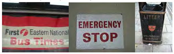
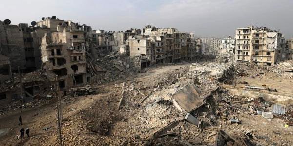
Figure 1: Examples of natural scene images where text detection is challenging due to lighting conditions, image quality, and non-planar objects (Figure 1 of Mancas-Thillou and Gosselin).

Detecting text in constrained, controlled environments can typically be accomplished by using heuristic-based approaches, such as exploiting gradient information or the fact that text is typically grouped into paragraphs and characters appear on a straight line. An example of such a heuristic-based text detector can be seen in my previous blog post on Detecting machine-readable zones in passport images.

Natural scene text detection is different though — and much more challenging.

Due to the proliferation of cheap digital cameras, and not to mention the fact that nearly every smartphone now has a camera, we need to be highly concerned with the conditions the image was captured under — and furthermore, what assumptions we can and cannot make. I’ve included a summarized version of the natural scene text detection challenges described by Celine Mancas-Thillou and Bernard Gosselin in their excellent 2017

paper, Natural Scene Text Understanding below:

• Image/sensor noise: Sensor noise from a handheld camera is typically higher than that of a traditional scanner. Additionally, low-priced cameras will typically interpolate the pixels of raw sensors to produce real colors.
• Viewing angles: Natural scene text can naturally have viewing angles that are not parallel to the text, making the text harder to recognize.
• Blurring: Uncontrolled environments tend to have blur, especially if the end user is utilizing a smartphone that does not have some form of stabilization.
• Lighting conditions: We cannot make any assumptions regarding our lighting conditions in natural scene images. It may be near dark, the flash on the camera may be on, or the sun may be shining brightly, saturating the entire image.
• Resolution: Not all cameras are created equal — we may be dealing with cameras with sub-par resolution.
• Non-paper objects: Most, but not all, paper is not reflective (at least in context of paper you are trying to scan). Text in natural scenes may be reflective, including logos, signs, etc.
• Non-planar objects: Consider what happens when you wrap text around a bottle — the text on the surface becomes distorted and deformed. While humans may still be able to easily “detect” and read the text, our algorithms will struggle. We need to be able to handle such use cases.
• Unknown layout: We cannot use any a priori information to give our algorithms “clues” as to where the text resides.

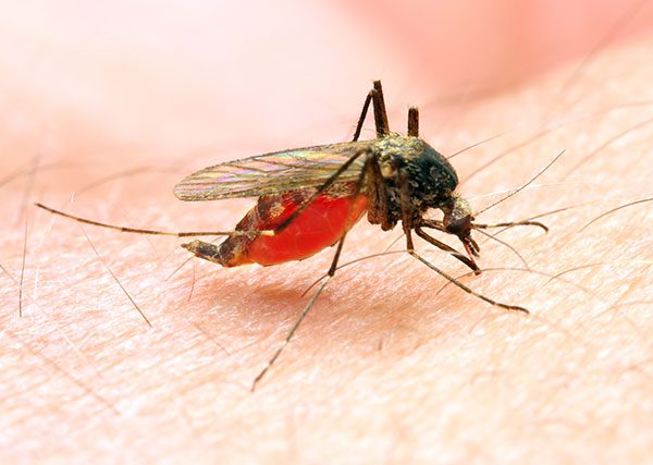
As we’ll learn, OpenCV’s text detector implementation of EAST is quite robust, capable of localizing text even when it’s blurred, reflective, or partially obscured:

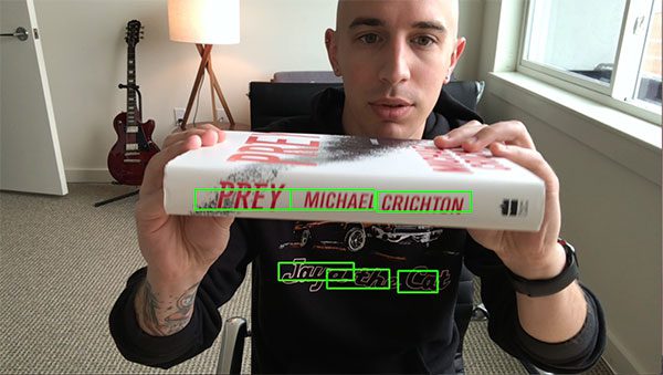
Figure 2: OpenCV’s EAST scene text detector will detect even in blurry and obscured images.

I would suggest reading Mancas-Thillou and Gosselin’s work if you are further interested in the challenges associated with text detection in natural scene images.

The EAST deep learning text detector

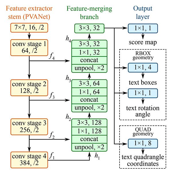
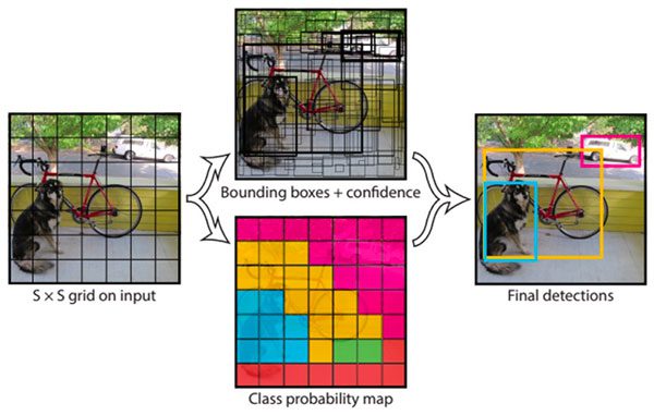
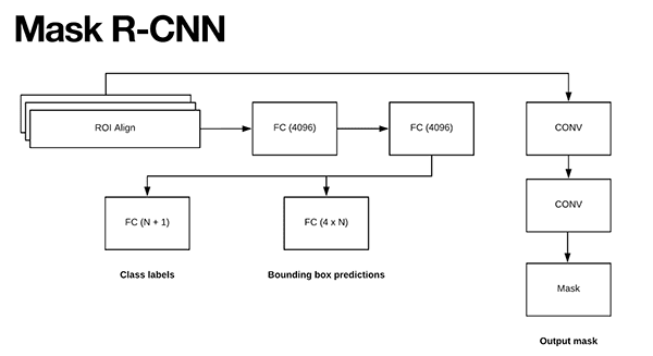
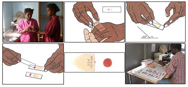
Figure 3: The structure of the EAST text detection Fully-Convolutional Network (Figure 3 of Zhou et al.).

With the release of OpenCV 3.4.2 and OpenCV 4, we can now use a deep learning-based text detector called EAST, which is based on Zhou et al.’s 2017

paper, EAST: An Efficient and Accurate Scene Text Detector.

We call the algorithm “EAST” because it’s an: Efficient and Accurate Scene Text detection pipeline.

The EAST pipeline is capable of predicting words and lines of text at arbitrary orientations on 720p images, and furthermore, can run at 13 FPS, according to the authors.

Perhaps most importantly, since the deep learning model is end-to-end, it is possible to sidestep computationally expensive sub-algorithms that other text detectors typically apply, including candidate aggregation and word partitioning.

To build and train such a deep learning model, the EAST method utilizes novel, carefully designed loss functions.

For more details on EAST, including architecture design and training methods, be sure to refer to the publication by the authors.

Project structure

To start, be sure to grab the source code + images to today’s post by visiting the “Downloads” section. From there, simply use the

tree

$ tree --dirsfirst
.
├── images
│   ├── car_wash.png
│   ├── lebron_james.jpg
│   └── sign.jpg
├── frozen_east_text_detection.pb
├── text_detection.py
└── text_detection_video.py

1 directory, 6 files

Notice that I’ve provided three sample pictures in the

images/

We’ll be reviewing two

.py

• text_detection.py

   : Detects text in static images.

• text_detection_video.py

   : Detects text via your webcam or input video files.

Both scripts make use of the serialized EAST model (

frozen_east_text_detection.pb

Implementation notes

The text detection implementation I am including today is based on OpenCV’s official C++ example; however, I must admit that I had a bit of trouble when converting it to Python.

To start, there are no

Point2f

RotatedRect

Secondly, the

NMSBoxes

NMSBoxes

I got around this issue my using my own non-maxima suppression implementation in imutils, but again, I don’t believe these two are 100% interchangeable as it appears

NMSBoxes

Given all that, I’ve tried my best to provide you with the best OpenCV text detection implementation I could, using the working functions and resources I had. If you have any improvements to the method please do feel free to share them in the comments below.

Implementing our text detector with OpenCV

Before we get started, I want to point out that you will need at least OpenCV 3.4.2 (or OpenCV 4) installed on your system to utilize OpenCV’s EAST text detector, so if you haven’t already installed OpenCV 3.4.2 or better on your system, please refer to my OpenCV install guides.

Next, make sure you have

imutils

$ pip install --upgrade imutils

At this point your system is now configured, so open up

text_detection.py

# import the necessary packages
from imutils.object_detection import non_max_suppression
import numpy as np
import argparse
import time
import cv2

# construct the argument parser and parse the arguments
ap = argparse.ArgumentParser()
ap.add_argument("-i", "--image", type=str,
	help="path to input image")
ap.add_argument("-east", "--east", type=str,
	help="path to input EAST text detector")
ap.add_argument("-c", "--min-confidence", type=float, default=0.5,
	help="minimum probability required to inspect a region")
ap.add_argument("-w", "--width", type=int, default=320,
	help="resized image width (should be multiple of 32)")
ap.add_argument("-e", "--height", type=int, default=320,
	help="resized image height (should be multiple of 32)")
args = vars(ap.parse_args())

To begin, we import our required packages and modules on Lines 2-6. Notably we import NumPy, OpenCV, and my implementation of 

non_max_suppression

imutils.object_detection

We then proceed to parse five command line arguments on Lines 9-20:

• --image

   : The path to our input image.

• --east

   : The EAST scene text detector model file path.

• --min-confidence

   : Probability threshold to determine text. Optional with

  default=0.5

   .

• --width

   : Resized image width — must be multiple of 32. Optional with

  default=320

   .

• --height

   : Resized image height — must be multiple of 32. Optional with

  default=320

   .

Important: The EAST text requires that your input image dimensions be multiples of 32, so if you choose to adjust your

--width

--height

From there, let’s load our image and resize it:

# load the input image and grab the image dimensions
image = cv2.imread(args["image"])
orig = image.copy()
(H, W) = image.shape[:2]

# set the new width and height and then determine the ratio in change
# for both the width and height
(newW, newH) = (args["width"], args["height"])
rW = W / float(newW)
rH = H / float(newH)

# resize the image and grab the new image dimensions
image = cv2.resize(image, (newW, newH))
(H, W) = image.shape[:2]

On Lines 23 and 24, we load and copy our input image.

From there, Lines 30 and 31 determine the ratio of the original image dimensions to new image dimensions (based on the command line argument provided for

--width

--height

Then we resize the image, ignoring aspect ratio (Line 34).

In order to perform text detection using OpenCV and the EAST deep learning model, we need to extract the output feature maps of two layers:

# define the two output layer names for the EAST detector model that
# we are interested -- the first is the output probabilities and the
# second can be used to derive the bounding box coordinates of text
layerNames = [
	"feature_fusion/Conv_7/Sigmoid",
	"feature_fusion/concat_3"]

We construct a list of

layerNames

1. The first layer is our output sigmoid activation which gives us the probability of a region containing text or not.
2. The second layer is the output feature map that represents the “geometry” of the image — we’ll be able to use this geometry to derive the bounding box coordinates of the text in the input image

Let’s load the OpenCV’s EAST text detector:

# load the pre-trained EAST text detector
print("[INFO] loading EAST text detector...")
net = cv2.dnn.readNet(args["east"])

# construct a blob from the image and then perform a forward pass of
# the model to obtain the two output layer sets
blob = cv2.dnn.blobFromImage(image, 1.0, (W, H),
	(123.68, 116.78, 103.94), swapRB=True, crop=False)
start = time.time()
net.setInput(blob)
(scores, geometry) = net.forward(layerNames)
end = time.time()

# show timing information on text prediction
print("[INFO] text detection took {:.6f} seconds".format(end - start))

We load the neural network into memory using

cv2.dnn.readNet

args

Then we prepare our image by converting it to a

blob

To predict text we can simply set the

blob

net.forward

print

By supplying

layerNames

net.forward

• The output

  geometry

    map used to derive the bounding box coordinates of text in our input images
• And similarly, the

  scores

    map, containing the probability of a given region containing text

We’ll need to loop over each of these values, one-by-one:

# grab the number of rows and columns from the scores volume, then
# initialize our set of bounding box rectangles and corresponding
# confidence scores
(numRows, numCols) = scores.shape[2:4]
rects = []
confidences = []

# loop over the number of rows
for y in range(0, numRows):
	# extract the scores (probabilities), followed by the geometrical
	# data used to derive potential bounding box coordinates that
	# surround text
	scoresData = scores[0, 0, y]
	xData0 = geometry[0, 0, y]
	xData1 = geometry[0, 1, y]
	xData2 = geometry[0, 2, y]
	xData3 = geometry[0, 3, y]
	anglesData = geometry[0, 4, y]

We start off by grabbing the dimensions of the

scores

• rects

   : Stores the bounding box (x, y)-coordinates for text regions

• confidences

   : Stores the probability associated with each of the bounding boxes in

  rects

We’ll later be applying non-maxima suppression to these regions.

Looping over the rows begins on Line 68.

Lines 72-77 extract our scores and geometry data for the current row, 

y

Next, we loop over each of the column indexes for our currently selected row:

# loop over the number of columns
	for x in range(0, numCols):
		# if our score does not have sufficient probability, ignore it
		if scoresData[x] < args["min_confidence"]:
			continue

		# compute the offset factor as our resulting feature maps will
		# be 4x smaller than the input image
		(offsetX, offsetY) = (x * 4.0, y * 4.0)

		# extract the rotation angle for the prediction and then
		# compute the sin and cosine
		angle = anglesData[x]
		cos = np.cos(angle)
		sin = np.sin(angle)

		# use the geometry volume to derive the width and height of
		# the bounding box
		h = xData0[x] + xData2[x]
		w = xData1[x] + xData3[x]

		# compute both the starting and ending (x, y)-coordinates for
		# the text prediction bounding box
		endX = int(offsetX + (cos * xData1[x]) + (sin * xData2[x]))
		endY = int(offsetY - (sin * xData1[x]) + (cos * xData2[x]))
		startX = int(endX - w)
		startY = int(endY - h)

		# add the bounding box coordinates and probability score to
		# our respective lists
		rects.append((startX, startY, endX, endY))
		confidences.append(scoresData[x])

For every row, we begin looping over the columns on Line 80.

We need to filter out weak text detections by ignoring areas that do not have sufficiently high probability (Lines 82 and 83).

The EAST text detector naturally reduces volume size as the image passes through the network — our volume size is actually 4x smaller than our input image so we multiply by four to bring the coordinates back into respect of our original image.

I’ve included how you can extract the

angle

From there, Lines 97-105 derive the bounding box coordinates for the text area.

We then update our

rects

confidences

We’re almost finished!

The final step is to apply non-maxima suppression to our bounding boxes to suppress weak overlapping bounding boxes and then display the resulting text predictions:

# apply non-maxima suppression to suppress weak, overlapping bounding
# boxes
boxes = non_max_suppression(np.array(rects), probs=confidences)

# loop over the bounding boxes
for (startX, startY, endX, endY) in boxes:
	# scale the bounding box coordinates based on the respective
	# ratios
	startX = int(startX * rW)
	startY = int(startY * rH)
	endX = int(endX * rW)
	endY = int(endY * rH)

	# draw the bounding box on the image
	cv2.rectangle(orig, (startX, startY), (endX, endY), (0, 255, 0), 2)

# show the output image
cv2.imshow("Text Detection", orig)
cv2.waitKey(0)

As I mentioned in the previous section, I could not use the non-maxima suppression in my OpenCV 4 install (

cv2.dnn.NMSBoxes

Instead, I have used my non-maxima suppression implementation available in the

imutils

NMSBoxes

Lines 117-126 loop over our bounding

boxes

orig

orig

As a final implementation note I would like to mention that our two nested

for

scores

geometry

OpenCV text detection results

Are you ready to apply text detection to images?

Start by grabbing the “Downloads” for this blog post and unzip the files.

From there, you may execute the following command in your terminal (taking note of the two command line arguments):

$ python text_detection.py --image images/lebron_james.jpg \
	--east frozen_east_text_detection.pb
[INFO] loading EAST text detector...
[INFO] text detection took 0.142082 seconds

Your results should look similar to the following image:

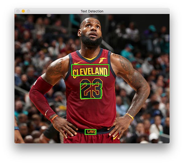
Figure 4: Famous basketball player, Lebron James’ jersey text is successfully recognized with OpenCV and EAST text detection.

Three text regions are identified on Lebron James.

Now let’s try to detect text of a business sign:

$ python text_detection.py --image images/car_wash.png \
	--east frozen_east_text_detection.pb
[INFO] loading EAST text detector...
[INFO] text detection took 0.142295 seconds

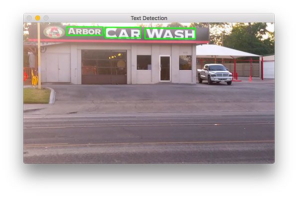
Figure 5: Text is easily recognized with Python and OpenCV using EAST in this natural scene of a car wash station.

And finally, we’ll try a road sign:

$ python text_detection.py --image images/sign.jpg \
	--east frozen_east_text_detection.pb
[INFO] loading EAST text detector...
[INFO] text detection took 0.141675 seconds

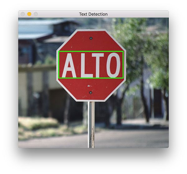
Figure 6: Scene text detection with Python + OpenCV and the EAST text detector successfully detects the text on this Spanish stop sign.

This scene contains a Spanish stop sign. The word, “ALTO” is correctly detected by OpenCV and EAST.

As you can tell, EAST is quite accurate and relatively fast taking approximately 0.14 seconds on average per image.

Text detection in video with OpenCV

Now that we’ve seen how to detect text in images, let’s move on to detecting text in video with OpenCV.

This explanation will be very brief; please refer to the previous section for details as needed.

Open up

text_detection_video.py

# import the necessary packages
from imutils.video import VideoStream
from imutils.video import FPS
from imutils.object_detection import non_max_suppression
import numpy as np
import argparse
import imutils
import time
import cv2

We begin by importing our packages. We’ll be using

VideoStream

FPS

For convenience, let’s define a new function to decode our predictions function — it will be reused for each frame and make our loop cleaner:

def decode_predictions(scores, geometry):
	# grab the number of rows and columns from the scores volume, then
	# initialize our set of bounding box rectangles and corresponding
	# confidence scores
	(numRows, numCols) = scores.shape[2:4]
	rects = []
	confidences = []

	# loop over the number of rows
	for y in range(0, numRows):
		# extract the scores (probabilities), followed by the
		# geometrical data used to derive potential bounding box
		# coordinates that surround text
		scoresData = scores[0, 0, y]
		xData0 = geometry[0, 0, y]
		xData1 = geometry[0, 1, y]
		xData2 = geometry[0, 2, y]
		xData3 = geometry[0, 3, y]
		anglesData = geometry[0, 4, y]

		# loop over the number of columns
		for x in range(0, numCols):
			# if our score does not have sufficient probability,
			# ignore it
			if scoresData[x] < args["min_confidence"]:
				continue

			# compute the offset factor as our resulting feature
			# maps will be 4x smaller than the input image
			(offsetX, offsetY) = (x * 4.0, y * 4.0)

			# extract the rotation angle for the prediction and
			# then compute the sin and cosine
			angle = anglesData[x]
			cos = np.cos(angle)
			sin = np.sin(angle)

			# use the geometry volume to derive the width and height
			# of the bounding box
			h = xData0[x] + xData2[x]
			w = xData1[x] + xData3[x]

			# compute both the starting and ending (x, y)-coordinates
			# for the text prediction bounding box
			endX = int(offsetX + (cos * xData1[x]) + (sin * xData2[x]))
			endY = int(offsetY - (sin * xData1[x]) + (cos * xData2[x]))
			startX = int(endX - w)
			startY = int(endY - h)

			# add the bounding box coordinates and probability score
			# to our respective lists
			rects.append((startX, startY, endX, endY))
			confidences.append(scoresData[x])

	# return a tuple of the bounding boxes and associated confidences
	return (rects, confidences)

On Line 11 we define

decode_predictions

1. The bounding box coordinates of a text region
2. And the probability of a text region detection

This dedicated function will make the code easier to read and manage later on in this script.

Let’s parse our command line arguments:

# construct the argument parser and parse the arguments
ap = argparse.ArgumentParser()
ap.add_argument("-east", "--east", type=str, required=True,
	help="path to input EAST text detector")
ap.add_argument("-v", "--video", type=str,
	help="path to optinal input video file")
ap.add_argument("-c", "--min-confidence", type=float, default=0.5,
	help="minimum probability required to inspect a region")
ap.add_argument("-w", "--width", type=int, default=320,
	help="resized image width (should be multiple of 32)")
ap.add_argument("-e", "--height", type=int, default=320,
	help="resized image height (should be multiple of 32)")
args = vars(ap.parse_args())

Our command line arguments are parsed on Lines 69-80:

• --east

   : The EAST scene text detector model file path.

• --video

   : The path to our input video. Optional — if a video path is provided then the webcam will not be used.

• --min-confidence

   : Probability threshold to determine text. Optional with

  default=0.5

   .

• --width

   : Resized image width (must be multiple of 32). Optional with

  default=320

   .

• --height

   : Resized image height (must be multiple of 32). Optional with

  default=320

   .

The primary change from the image-only script in the previous section (in terms of command line arguments) is that I’ve substituted the

--image

--video

Important: The EAST text requires that your input image dimensions be multiples of 32, so if you choose to adjust your

--width

--height

Next, we’ll perform important initializations which mimic the previous script:

# initialize the original frame dimensions, new frame dimensions,
# and ratio between the dimensions
(W, H) = (None, None)
(newW, newH) = (args["width"], args["height"])
(rW, rH) = (None, None)

# define the two output layer names for the EAST detector model that
# we are interested -- the first is the output probabilities and the
# second can be used to derive the bounding box coordinates of text
layerNames = [
	"feature_fusion/Conv_7/Sigmoid",
	"feature_fusion/concat_3"]

# load the pre-trained EAST text detector
print("[INFO] loading EAST text detector...")
net = cv2.dnn.readNet(args["east"])

The height/width and ratio initializations on Lines 84-86 will allow us to properly scale our bounding boxes later on.

Our output layer names are defined and we load our pre-trained EAST text detector on Lines 91-97.

The following block sets up our video stream and frames per second counter:

# if a video path was not supplied, grab the reference to the web cam
if not args.get("video", False):
	print("[INFO] starting video stream...")
	vs = VideoStream(src=0).start()
	time.sleep(1.0)

# otherwise, grab a reference to the video file
else:
	vs = cv2.VideoCapture(args["video"])

# start the FPS throughput estimator
fps = FPS().start()

Our video stream is set up for either:

• A webcam (Lines 100-103)
• Or a video file (Lines 106-107)

From there we initialize our frames per second counter on Line 110 and begin looping over incoming frames:

# loop over frames from the video stream
while True:
	# grab the current frame, then handle if we are using a
	# VideoStream or VideoCapture object
	frame = vs.read()
	frame = frame[1] if args.get("video", False) else frame

	# check to see if we have reached the end of the stream
	if frame is None:
		break

	# resize the frame, maintaining the aspect ratio
	frame = imutils.resize(frame, width=1000)
	orig = frame.copy()

	# if our frame dimensions are None, we still need to compute the
	# ratio of old frame dimensions to new frame dimensions
	if W is None or H is None:
		(H, W) = frame.shape[:2]
		rW = W / float(newW)
		rH = H / float(newH)

	# resize the frame, this time ignoring aspect ratio
	frame = cv2.resize(frame, (newW, newH))

We begin looping over video/webcam frames on Line 113.

Our frame is resized, maintaining aspect ratio (Line 124). From there, we grab dimensions and compute the scaling ratios (Lines 129-132). We then resize the frame again (must be a multiple of 32), this time ignoring aspect ratio since we have stored the ratios for safe keeping (Line 135).

Inference and drawing text region bounding boxes take place on the following lines:

# construct a blob from the frame and then perform a forward pass
	# of the model to obtain the two output layer sets
	blob = cv2.dnn.blobFromImage(frame, 1.0, (newW, newH),
		(123.68, 116.78, 103.94), swapRB=True, crop=False)
	net.setInput(blob)
	(scores, geometry) = net.forward(layerNames)

	# decode the predictions, then  apply non-maxima suppression to
	# suppress weak, overlapping bounding boxes
	(rects, confidences) = decode_predictions(scores, geometry)
	boxes = non_max_suppression(np.array(rects), probs=confidences)

	# loop over the bounding boxes
	for (startX, startY, endX, endY) in boxes:
		# scale the bounding box coordinates based on the respective
		# ratios
		startX = int(startX * rW)
		startY = int(startY * rH)
		endX = int(endX * rW)
		endY = int(endY * rH)

		# draw the bounding box on the frame
		cv2.rectangle(orig, (startX, startY), (endX, endY), (0, 255, 0), 2)

In this block we:

• Detect text regions using EAST via creating a

  blob

    and passing it through the network (Lines 139-142)
• Decode the predictions and apply NMS (Lines 146 and 147). We use the

  decode_predictions

    function defined previously in this script and my imutils

  non_max_suppression

    convenience function.
• Loop over bounding boxes and draw them on the

  frame

    (Lines 150-159). This involves scaling the boxes by the ratios gathered earlier.

From there we’ll close out the frame processing loop as well as the script itself:

# update the FPS counter
	fps.update()

	# show the output frame
	cv2.imshow("Text Detection", orig)
	key = cv2.waitKey(1) & 0xFF

	# if the `q` key was pressed, break from the loop
	if key == ord("q"):
		break

# stop the timer and display FPS information
fps.stop()
print("[INFO] elasped time: {:.2f}".format(fps.elapsed()))
print("[INFO] approx. FPS: {:.2f}".format(fps.fps()))

# if we are using a webcam, release the pointer
if not args.get("video", False):
	vs.stop()

# otherwise, release the file pointer
else:
	vs.release()

# close all windows
cv2.destroyAllWindows()

We update our

fps

We show the output of EAST text detection on Line 165 and handle keypresses (Lines 166-170). If “q” is pressed for “quit”, we

break

Video text detection results

To apply text detection to video with OpenCV, be sure to use the “Downloads” section of this blog post.

From there, open up a terminal and execute the following command (which will fire up your webcam since we aren’t supplying a

--video

$ python text_detection_video.py --east frozen_east_text_detection.pb 
[INFO] loading EAST text detector...
[INFO] starting video stream...
[INFO] elasped time: 59.76
[INFO] approx. FPS: 8.85

Our OpenCV text detection video script achieves 7-9 FPS.

This result is not quite as fast as the authors reported (13 FPS); however, we are using Python instead of C++. By optimizing our for loops with Cython, we should be able to increase the speed of our text detection pipeline.

Summary

In today’s blog post, we learned how to use OpenCV’s new EAST text detector to automatically detect the presence of text in natural scene images.

The text detector is not only accurate, but it’s capable of running in near real-time at approximately 13 FPS on 720p images.

In order to provide an implementation of OpenCV’s EAST text detector, I needed to convert OpenCV’s C++ example; however, there were a number of challenges I encountered, such as:

1. Not being able to use OpenCV’s

   NMSBoxes

     for non-maxima suppression and instead having to use my implementation from

   imutils

    .
2. Not being able to compute a true rotated bounding box due to the lack of Python bindings for

   RotatedRect

    .

I tried to keep my implementation as close to OpenCV’s as possible, but keep in mind that my version is not 100% identical to the C++ version and that there may be one or two small problems that will need to be resolved over time.

In any case, I hope you enjoyed today’s tutorial on text detection with OpenCV!

To download the source code to this tutorial, and start applying text detection to your own images, just enter your email address in the form below.

Downloads:

If you would like to download the code and images used in this post, please enter your email address in the form below. Not only will you get a .zip of the code, I’ll also send you a FREE 17-page Resource Guide on Computer Vision, OpenCV, and Deep Learning. Inside you'll find my hand-picked tutorials, books, courses, and libraries to help you master CV and DL! Sound good? If so, enter your email address and I’ll send you the code immediately!

Email address:

The post OpenCV Text Detection (EAST text detector) appeared first on PyImageSearch.

In this tutorial, you will learn how to apply neural style transfer to both images and real-time video using OpenCV, Python, and deep learning. By the end of this guide, you’ll be able to generate beautiful works of art with neural style transfer.

The original neural style transfer algorithm was introduced by Gatys et al. in their 2015 paper, A Neural Algorithm of Artistic Style (in fact, this is the exact algorithm that I teach you how to implement and train from scratch inside Deep Learning for Computer Vision with Python).

In 2016, Johnson et al. published Perceptual Losses for Real-Time Style Transfer and Super- Resolution, which frames neural style transfer as a super-resolution-like problem using perceptual loss. The end result is a neural style transfer algorithm which is up to three orders of magnitude faster than the Gatys et al. method (there are a few downsides though and I’ll be discussing them later in the guide).

In the rest of this post you will learn how to apply the neural style transfer algorithm to your own images and video streams.

To learn how to apply neural style transfer using OpenCV and Python, just keep reading!

Neural Style Transfer with OpenCV

In the remainder of today’s guide I will be demonstrating how you can apply the neural style transfer algorithm using OpenCV and Python to generate your own works of art.

The method I’m discussing here today is capable of running in near real-time on a CPU and is fully capable of obtaining super real-time performance on your GPU.

We’ll start with a brief discussion of neural style transfer, including what it is and how it works.

From there we’ll utilize OpenCV and Python to actually apply neural style transfer.

What is neural style transfer?

Figure 1: Neural style transfer with OpenCV example. Our content image (left). Style image (middle). Stylized output (right).

Neural style transfer is the process of:

1. Taking the style of one image
2. And then applying it to the content of another image

An example of the neural style transfer process can be seen in Figure 1. On the left we have our content image — a serene view of myself enjoying a beer on top of a mountain in the Black Forest of Germany, overlooking the town of Baden.

In the middle is our style image, Vincent van Gogh’s famous The Starry Night.

And on the right is the output of applying the style of van Gogh’s Starry Night to the content of my photo of Germany’s Black Forest. Notice how we have retained the content of the rolling hills, forest, myself, and even the beers, but have applied the style of Starry Night — it’s as if Van Gogh had applied his masterful paint strokes to our scenic view!

The question is, how do we define a neural network to perform neural style transfer?

Is that even possible?

You bet it is — and we’ll be discussing how neural style transfer is made possible in the next section.

How does neural style transfer work?

Figure 2: Neural Style Transfer with OpenCV possible (Figure 1 of Gatys et. al. 2015).

At this point you’re probably scratching your head and thinking something along the lines of: “How do we define a neural network to perform style transfer?”

Interestingly, the original 2015 paper by Gatys et al. proposed a neural style transfer algorithm that does not require a new architecture at all. Instead, we can take a pre-trained network (typically on ImageNet) and define a loss function that will enable us to achieve our end goal of style transfer and then optimize over that loss function.

Therefore, the question isn’t “What neural network do we use?” but rather “What loss function do we use?”

The answer is a three-component loss function, including:

1. Content loss
2. Style loss
3. Total-variation loss

Each component is individually computed and then combined in a single meta-loss function. By minimizing the meta-loss function we will be in turn jointly optimizing the content, style, and total-variation loss as well.

While the Gatys et al. method produced beautiful neural style transfer results, the problem was that it was quite slow.

Johnson et al. (2016) built on the work of Gatys et al., proposing a neural style transfer algorithm that is up to three orders of magnitude faster. The Johnson et al. method frames neural style transfer as a super-resolution-like problem based on perceptual loss functions.

While the Johnson et al. method is certainly fast, the biggest downside is that you cannot arbitrarily select your style images like you could in the Gatys et al. method.

Instead, you first need to explicitly train a network to reproduce the style of your desired image. Once the network is trained, you can then apply it to any content image you wish. You should see the Johnson et al. method as a more of an “investment” in your style image — you better like your style image as you’ll be training your own network to reproduce its style on content images.

Johnson et al. provide documentation on how to train your own neural style transfer models on their official GitHub page.

Finally, it’s also worth nothing that that in Ulyanov et al.’s 2017 publication, Instance Normalization: The Missing Ingredient for Fast Stylization, it was found that swapping batch normalization for instance normalization (and applying instance normalization at both training and testing), leads to even faster real-time performance and arguably more aesthetically pleasing results as well.

I have included both the models used by Johnson et al. in their ECCV paper along with the Ulyanov et al. models in the “Downloads” section of this post — be sure to download them so you can follow along with the remainder of this guide.

And if you’re interested in learning more about how neural style transfer works, be sure to refer to my book, Deep Learning for Computer Vision with Python.

Project structure

Today’s project includes a number of files which you can grab from the “Downloads” section.

Once you’ve grabbed the scripts + models + images, you can inspect the project structure with the

tree

$ tree --dirsfirst
.
├── images
│   ├── baden_baden.jpg
│   ├── giraffe.jpg
│   ├── jurassic_park.jpg
│   └── messi.jpg
├── models
│   ├── eccv16
│   │   ├── composition_vii.t7
│   │   ├── la_muse.t7
│   │   ├── starry_night.t7
│   │   └── the_wave.t7
│   └── instance_norm
│       ├── candy.t7
│       ├── feathers.t7
│       ├── la_muse.t7
│       ├── mosaic.t7
│       ├── starry_night.t7
│       ├── the_scream.t7
│       └── udnie.t7
├── neural_style_transfer.py
├── neural_style_transfer_examine.py
└── neural_style_transfer_video.py

4 directories, 18 files

Once you use the “Downloads” section of the blog post to grab the .zip, you won’t need to go hunting for anything else online. I’ve provided a handful of test

images/

models/

Implementing neural style transfer

Let’s get started implementing neural style transfer with OpenCV and Python.

Open up your

neural_style_transfer.py

# import the necessary packages
import argparse
import imutils
import time
import cv2

# construct the argument parser and parse the arguments
ap = argparse.ArgumentParser()
ap.add_argument("-m", "--model", required=True,
	help="neural style transfer model")
ap.add_argument("-i", "--image", required=True,
	help="input image to apply neural style transfer to")
args = vars(ap.parse_args())

First, we import our required packages and parse command line arguments.

Our notable imports are:

• imutils: This package is pip-installable via

  pip install --upgrade imutils

   . I recently released

  imutils==0.5.1

   , so don’t forget to upgrade!
• OpenCV: You need OpenCV 3.4 or better in order to use today’s code. You can install OpenCV 4 using my tutorials for Ubuntu and macOS.

We have two required command line arguments for this script:

• --model

   : The neural style transfer model path. I’ve included 11 pre-trained models for you to use in the “Downloads”.

• --image

   : Our input image which we’ll apply the neural style to. I’ve included 4 sample images. Feel free to experiment with your own as well!

You do not have to change the command line argument code — the arguments are passed and processed at runtime. If you aren’t familiar with how this works, be sure to read my command line arguments + argparse blog post.

Now comes the fun part — we’re going to load our image + model and then compute neural style transfer:

# load the neural style transfer model from disk
print("[INFO] loading style transfer model...")
net = cv2.dnn.readNetFromTorch(args["model"])

# load the input image, resize it to have a width of 600 pixels, and
# then grab the image dimensions
image = cv2.imread(args["image"])
image = imutils.resize(image, width=600)
(h, w) = image.shape[:2]

# construct a blob from the image, set the input, and then perform a
# forward pass of the network
blob = cv2.dnn.blobFromImage(image, 1.0, (w, h),
	(103.939, 116.779, 123.680), swapRB=False, crop=False)
net.setInput(blob)
start = time.time()
output = net.forward()
end = time.time()

In this code block we proceed to:

• Load a pre-trained neural style transfer model into memory as

  net

    (Line 17).
• Load the input

  image

    and resize it (Lines 21 and 22).
• Construct a

  blob

    by performing mean subtraction (Lines 27 and 28). Read about

  cv2.dnn.blobFromImage

    and how it works in my previous blog post.
• Perform a 

  forward

    pass to obtain an 

  output

    image (i.e., the result of the neural style transfer process) on Line 31. I’ve also surrounded this line with timestamps for benchmarking purposes.

Next, it is critical that we post-process the

output

# reshape the output tensor, add back in the mean subtraction, and
# then swap the channel ordering
output = output.reshape((3, output.shape[2], output.shape[3]))
output[0] += 103.939
output[1] += 116.779
output[2] += 123.680
output /= 255.0
output = output.transpose(1, 2, 0)

For the particular image I’m using for this example, the

output

(1, 3, 452, 600)

• The

  1

    indicates that we passed a batch size of one (i.e., just our single image) through the network.
• OpenCV is using channels-first ordering here, indicating there are

  3

    channels in the output image.
• The final two values in the output shape are the number of rows (height) and number of columns (width).

We reshape the matrix to simply be

(3, H, W)

1. Adding back in the mean values we previously subtracted (Lines 37-39).
2. Scaling (Line 40).
3. Transposing the matrix to be channels-last ordering (Line 41).

The final step is to show the output of the neural style transfer process to our screen:

# show information on how long inference took
print("[INFO] neural style transfer took {:.4f} seconds".format(
	end - start))

# show the images
cv2.imshow("Input", image)
cv2.imshow("Output", output)
cv2.waitKey(0)

Neural style transfer results

In order to replicate my results, you will need to grab the “Downloads” for this blog post.

Once you’ve grabbed the files, open up terminal and execute the following command:

$ python neural_style_transfer.py --image images/giraffe.jpg \
	--model models/eccv16/the_wave.t7
[INFO] loading style transfer model...
[INFO] neural style transfer took 0.3152 seconds

Figure 3: Neural Style Transfer with OpenCV applied to a picture of me feeding a giraffe. The output is stylized from The Great Wave Off Kanagawa which you can see in the top-right corner.

Now, simply change the command line arguments to use a screen capture from my favorite movie, Jurassic Park, as the content image, and then The Scream style model:

$ python neural_style_transfer.py --image images/jurassic_park.jpg \
	--model models/instance_norm/the_scream.t7
[INFO] loading style transfer model...
[INFO] neural style transfer took 0.1202 seconds

Figure 4: A Jurassic Park movie frame undergoes Neural Style Transfer using OpenCV. The Scream style is applied to the image producing an artistic effect.

And changing the command line arguments in your terminal once more:

$ python neural_style_transfer.py --image images/messi.jpg \
	--model models/instance_norm/udnie.t7 
[INFO] loading style transfer model...
[INFO] neural style transfer took 0.1495 seconds

Figure 5: Using the artist Francis Picabia’s famous Udnie, Young American Girl oil painting, an image of Lionel Messi, Argentinian soccer player, undergoes Neural Style Transfer with OpenCV.

Figure 5 is arguably my favorite — it just feels like it could be printed and hung on a wall in a sports bar.

In these three examples, we’ve created deep learning art! In the terminal output, the time elapsed to compute the output image is shown — each CNN model is a little bit different and you should expect different timings for each of the models.

Challenge! Can you create fancy deep learning artwork with neural style transfer? I’d love to see you tweet your artwork results — just use the hashtag, #neuralstyletransfer and mention me in the tweet (@PyImageSearch). Also, be sure to give credit to the artists and photographers — tag them if they are on Twitter as well.

Real-time neural style transfer

Now that we’ve learned how to apply neural style transfer to single images, let’s learn how to apply the process to (near) real-time video as well.

The process is quite similar to performing neural style transfer on a static image. In this script, we’ll:

• Utilize a special Python iterator which will allow us to cycle over all available neural style transfer models in our

  models

    path.
• Start our webcam video stream — our webcam frames will be processed in (near) real-time. Slower systems may lag quite a bit for certain larger models.
• Loop over incoming frames.
• Perform neural style transfer on the frame, post-process the output, and display the result to the screen (you’ll recognize this from above as it is nearly identical).
• If the user presses the “n” key on their keyboard, we’ll utilize the iterator to cycle to the next neural style transfer model without having to stop/restart the script.

Without further ado, let’s get to it.

Open up your

neural_style_transfer_video.py

# import the necessary packages
from imutils.video import VideoStream
from imutils import paths
import itertools
import argparse
import imutils
import time
import cv2

# construct the argument parser and parse the arguments
ap = argparse.ArgumentParser()
ap.add_argument("-m", "--models", required=True,
	help="path to directory containing neural style transfer models")
args = vars(ap.parse_args())

We begin by importing required packages/modules.

From there, we just need the path to our

models/

--models

argparse

Next, let’s create our model path iterator:

# grab the paths to all neural style transfer models in our 'models'
# directory, provided all models end with the '.t7' file extension
modelPaths = paths.list_files(args["models"], validExts=(".t7",))
modelPaths = sorted(list(modelPaths))

# generate unique IDs for each of the model paths, then combine the
# two lists together
models = list(zip(range(0, len(modelPaths)), (modelPaths)))

# use the cycle function of itertools that can loop over all model
# paths, and then when the end is reached, restart again
modelIter = itertools.cycle(models)
(modelID, modelPath) = next(modelIter)

Once we begin processing frames in a

while

To construct our model iterator, we:

• Grab and sort paths to all neural style transfer models (Lines 18 and 19).
• Assign a unique ID to each (Line 23).
• Use

  itertools

    and

  cycle

    to create an iterator (Line 27). Essentially,

  cycle

    allows us to create a circular list which when you reach the end of it, starts back at the beginning.

Calling the 

next

modelIter

modelID

modelPath

If you are new to Python iterators or iterators in general (most programming languages implement them), then be sure to give this article by RealPython a read.

Let’s load the first neural style transfer model and initialize our video stream:

# load the neural style transfer model from disk
print("[INFO] loading style transfer model...")
net = cv2.dnn.readNetFromTorch(modelPath)

# initialize the video stream, then allow the camera sensor to warm up
print("[INFO] starting video stream...")
vs = VideoStream(src=0).start()
time.sleep(2.0)
print("[INFO] {}. {}".format(modelID + 1, modelPath))

On Line 32, we read the first neural style transfer model using its path.

Then on Lines 36 and 37, we initialize our video stream so we can grab frames from our webcam.

Let’s begin looping over frames:

# loop over frames from the video file stream
while True:
	# grab the frame from the threaded video stream
	frame = vs.read()

	# resize the frame to have a width of 600 pixels (while
	# maintaining the aspect ratio), and then grab the image
	# dimensions
	frame = imutils.resize(frame, width=600)
	orig = frame.copy()
	(h, w) = frame.shape[:2]

	# construct a blob from the frame, set the input, and then perform a
	# forward pass of the network
	blob = cv2.dnn.blobFromImage(frame, 1.0, (w, h),
		(103.939, 116.779, 123.680), swapRB=False, crop=False)
	net.setInput(blob)
	output = net.forward()

Our

while

Lines 43-57 are nearly identical to the previous script we reviewed with the only exception being that we load a frame from the video stream rather than an image file on disk.

Essentially we grab the

frame

blob

There’s a lot of computation going on behind the scenes here in the CNN. If you’re curious how to train your own neural style transfer model with Keras, be sure to refer to my book, Deep Learning for Computer Vision with Python.

Next, we’ll post-process and display the

output

# reshape the output tensor, add back in the mean subtraction, and
	# then swap the channel ordering
	output = output.reshape((3, output.shape[2], output.shape[3]))
	output[0] += 103.939
	output[1] += 116.779
	output[2] += 123.680
	output /= 255.0
	output = output.transpose(1, 2, 0)

	# show the original frame along with the output neural style
	# transfer
	cv2.imshow("Input", frame)
	cv2.imshow("Output", output)
	key = cv2.waitKey(1) & 0xFF

Again, Lines 61-66 are identical to the static image neural style script above where I explained these lines in detail. These lines are critical to you seeing the correct result. Our output image is “de-processed” by reshaping, mean addition (since we subtracted the mean earlier), rescaling, and transposing.

The output of our neural style transfer is shown on Lines 70 and 71, where both the original and processed frames are displayed on the screen.

We also capture keypresses on Line 72. The keys are processed in the next block:

# if the `n` key is pressed (for "next"), load the next neural
	# style transfer model
	if key == ord("n"):
		# grab the next neural style transfer model model and load it
		(modelID, modelPath) = next(modelIter)
		print("[INFO] {}. {}".format(modelID + 1, modelPath))
		net = cv2.dnn.readNetFromTorch(modelPath)

	# otheriwse, if the `q` key was pressed, break from the loop
	elif key == ord("q"):
		break

# do a bit of cleanup
cv2.destroyAllWindows()
vs.stop()

There are two keys that will cause different behaviors while the script is running:

• “n”: Grabs the “next” neural style transfer model path + ID and loads it (Lines 76-80). If we’ve reached the last model, the iterator will cycle back to the beginning.
• “q”: Pressing the “q” key will “quit” the

  while

    loop (Lines 83 and 84).

Cleanup is then performed on the remaining lines.

Real-time neural style transfer results

Once you’ve used the “Downloads” section of this tutorial to download the source code and neural style transfer models, you can execute the following command to apply style transfer to your own video streams:

$ python neural_style_transfer_video.py --models models

***S3 GIF neural_style_transfer_animation.gif***

As you can see, it’s easy to cycle through the neural style transfer models using a single keypress.

I have included a short demo video of myself applying neural transfer below:

Where can I learn more about neural style transfer?

If you’re interested in learning more about neural style transfer, including the history, theory, and implementing your own custom neural style transfer pipeline with Keras, I would suggest you take a look at my book, Deep Learning for Computer Vision with Python:

Inside the book I discuss the Gatys et al. method in detail, including fully-documented Python + Keras code.

Using the methods discussed in the book, you’ll be able to apply neural style transfer to your own style and content images.

Inside the book you’ll also find:

• Super practical walkthroughs that present solutions to actual, real-world image classification problems, challenges, and competitions.
• Hands-on tutorials (with lots of code) that not only show you the algorithms behind deep learning for computer vision but their implementations as well.
• A no-nonsense teaching style that is guaranteed to help you master deep learning for image understanding and visual recognition.

To learn more about the book (and grab your set of free sample chapters + table of contents), just use this link!

Summary

In today’s blog post you learned how to apply neural style transfer to both images and video using OpenCV and Python.

Specifically, we utilized the models trained by Johnson et al. in their 2016 publication on neural style transfer — for your convenience, I have included the models in the “Downloads” section of this blog post.

I hope you enjoyed today’s tutorial on neural style transfer!

Be sure to use Twitter and the comments section to post links to your own beautiful works of art — I can’t wait to see them!

To be notified when future blog posts are published here on PyImageSearch, just enter your email address in the form below!

Downloads:

If you would like to download the code and images used in this post, please enter your email address in the form below. Not only will you get a .zip of the code, I’ll also send you a FREE 17-page Resource Guide on Computer Vision, OpenCV, and Deep Learning. Inside you'll find my hand-picked tutorials, books, courses, and libraries to help you master CV and DL! Sound good? If so, enter your email address and I’ll send you the code immediately!

Email address:

The post Neural Style Transfer with OpenCV appeared first on PyImageSearch.

In this tutorial, you will learn how to perform semantic segmentation using OpenCV, deep learning, and the ENet architecture. After reading today’s guide, you will be able to apply semantic segmentation to images and video using OpenCV.

Deep learning has helped facilitate unprecedented accuracy in computer vision, including image classification, object detection, and now even segmentation.

Traditional segmentation involves partitioning an image into parts (Normalized Cuts, Graph Cuts, Grab Cuts, superpixels, etc.); however, the algorithm has no actual understanding of what these parts represent.

Semantic segmentation algorithms on the other hand attempt to:

1. Partition the image into meaningful parts
2. While at the same time, associate every pixel in an input image with a class label (i.e., person, road, car, bus, etc.)

Semantic segmentation algorithms are super powerful and have many use cases, including self-driving cars — and in today’s post, I’ll be showing you how to apply semantic segmentation to road-scene images/video!

To learn how to apply semantic segmentation using OpenCV and deep learning, just keep reading!

Semantic segmentation with OpenCV and deep learning

In the first part of today’s blog post, we will discuss the ENet deep learning architecture.

From there, I’ll demonstrate how to use ENet to apply semantic segmentation to both images and video streams.

Along the way, I’ll be sharing example outputs from the segmentation so you can get a feel for what to expect when applying semantic segmentation to your own projects.

The ENet semantic segmentation architecture

Figure 1: The ENet deep learning semantic segmentation architecture. This figure is a combination of Table 1 and Figure 2 of Paszke et al.

The semantic segmentation architecture we’re using for this tutorial is ENet, which is based on Paszke et al.’s 2016 publication, ENet: A Deep Neural Network Architecture for Real-Time Semantic Segmentation.

One of the primary benefits of ENet is that it’s fast — up to 18x faster and requiring 79x fewer parameters with similar or better accuracy than larger models. The model size itself is only 3.2MB!

A single forward pass on a CPU took 0.2 seconds on my machine — if I were to use a GPU this segmentation network could run even faster. Paszke et al. trained that dataset on The Cityscapes Dataset, a semantic, instance-wise, dense pixel annotation of 20-30 classes (depending on which model you’re using).

As the name suggests, the Cityscapes dataset includes examples of images that can be used for urban scene understanding, including self- driving vehicles.

The particular model we’re using is trained on 20 classes, including:

In the rest of this blog post, you’ll learn how to apply semantic segmentation to extract a dense, pixel-wise map of each of these classes in both images and video streams.

If you’re interested in training your own ENet models for segmentation on your own custom datasets, be sure to refer to this page where the authors have provided a tutorial on how to do so.

Project structure

Today’s project can be obtained from the “Downloads” section of this blog post. Let’s take a look at our project structure using the

tree

$ tree --dirsfirst
.
├── enet-cityscapes
│   ├── enet-classes.txt
│   ├── enet-colors.txt
│   └── enet-model.net
├── images
│   ├── example_01.png
│   ├── example_02.jpg
│   ├── example_03.jpg
│   └── example_04.png
├── videos
│   ├── massachusetts.mp4
│   └── toronto.mp4
├── output
├── segment.py
└── segment_video.py

4 directories, 11 files

Our project has four directories:

• enet-cityscapes/

   : Contains our pre-trained deep learning model, classes list, and color labels to correspond with the classes.

• images/

   : A selection of four sample images to test our image segmentation script.

• videos/

   : Includes two sample videos for testing our deep learning segmentation video script.  Credits for these videos are listed in the “Video segmentation results” section.

• output/

   : For organizational purposes, I like to have my script save the processed videos to the

  output

    folder. I’m not including the output images/videos in the downloads as the file sizes are quite larger. You’ll need to use today’s code to generate them on your own.

Today we’ll be reviewing two Python scripts:

• segment.py

   : Performs deep learning semantic segmentation on a single image. We’ll walk through this script to learn how segmentation works and then test it on single images before moving on to video.

• segment_video.py

   : As the name suggests, this script will perform semantic segmentation on video.

Semantic segmentation in images with OpenCV

Let’s go ahead and get started — open up the

segment.py

# import the necessary packages
import numpy as np
import argparse
import imutils
import time
import cv2

We begin by importing necessary packages.

For this script, I recommend OpenCV 3.4.1 or higher. You can follow one of my installation tutorials — just be sure to specify which version of OpenCV you want to download and install as you follow the steps.

You’ll also need to install my package of OpenCV convenience functions, imutils — just use pip to install the package:

$ pip install --upgrade imutils

If you are using Python virtual environments don’t forget to use the

workon

pip

imutils

Moving on, let’s parse our command line arguments:

# construct the argument parse and parse the arguments
ap = argparse.ArgumentParser()
ap.add_argument("-m", "--model", required=True,
	help="path to deep learning segmentation model")
ap.add_argument("-c", "--classes", required=True,
	help="path to .txt file containing class labels")
ap.add_argument("-i", "--image", required=True,
	help="path to input image")
ap.add_argument("-l", "--colors", type=str,
	help="path to .txt file containing colors for labels")
ap.add_argument("-w", "--width", type=int, default=500,
	help="desired width (in pixels) of input image")
args = vars(ap.parse_args())

This script has five command line arguments, two of which are optional:

• --model

   : The path to our deep learning semantic segmentation model.

• --classes

   : The path to a text file containing class labels.

• --image

   : Our input image file path.

• --colors

   : Optional path to a colors text file. If no file is specified, random colors will be assigned to each class.

• --width

   : Optional desired image width. By default the value is

  500

   pixels.

If you aren’t familiar with the concept of

argparse

Let’s handle our parsing our class labels files and colors next:

# load the class label names
CLASSES = open(args["classes"]).read().strip().split("\n")

# if a colors file was supplied, load it from disk
if args["colors"]:
	COLORS = open(args["colors"]).read().strip().split("\n")
	COLORS = [np.array(c.split(",")).astype("int") for c in COLORS]
	COLORS = np.array(COLORS, dtype="uint8")

# otherwise, we need to randomly generate RGB colors for each class
# label
else:
	# initialize a list of colors to represent each class label in
	# the mask (starting with 'black' for the background/unlabeled
	# regions)
	np.random.seed(42)
	COLORS = np.random.randint(0, 255, size=(len(CLASSES) - 1, 3),
		dtype="uint8")
	COLORS = np.vstack([[0, 0, 0], COLORS]).astype("uint8")

We load our

CLASSES

args

If a pre-specified set of

COLORS

COLORS

For testing purposes (and since we have 20 classes), let’s create a pretty color lookup legend using OpenCV drawing functions:

# initialize the legend visualization
legend = np.zeros(((len(CLASSES) * 25) + 25, 300, 3), dtype="uint8")

# loop over the class names + colors
for (i, (className, color)) in enumerate(zip(CLASSES, COLORS)):
	# draw the class name + color on the legend
	color = [int(c) for c in color]
	cv2.putText(legend, className, (5, (i * 25) + 17),
		cv2.FONT_HERSHEY_SIMPLEX, 0.5, (0, 0, 255), 2)
	cv2.rectangle(legend, (100, (i * 25)), (300, (i * 25) + 25),
		tuple(color), -1)

Here we generate a legend visualization so we can easily visually associate a class label with a color. The legend consists of the class label and a colored rectangle next to it. This is quickly created by creating a canvas (Line 43) and dynamically building the legend with a loop (Lines 46-52). Drawing basics are covered in this blog post.

Here’s the result:

Figure 2: Our deep learning semantic segmentation class color legend generated with OpenCV.

The deep learning segmentation heavy lifting takes place in the next block:

# load our serialized model from disk
print("[INFO] loading model...")
net = cv2.dnn.readNet(args["model"])

# load the input image, resize it, and construct a blob from it,
# but keeping mind mind that the original input image dimensions
# ENet was trained on was 1024x512
image = cv2.imread(args["image"])
image = imutils.resize(image, width=args["width"])
blob = cv2.dnn.blobFromImage(image, 1 / 255.0, (1024, 512), 0,
	swapRB=True, crop=False)

# perform a forward pass using the segmentation model
net.setInput(blob)
start = time.time()
output = net.forward()
end = time.time()

# show the amount of time inference took
print("[INFO] inference took {:.4f} seconds".format(end - start))

To perform deep learning semantic segmentation of an image with Python and OpenCV, we:

• Load the model (Line 56).
• Construct a

  blob

    (Lines 61-64).The ENet model we are using in this blog post was trained on input images with 1024×512 resolution — we’ll use the same here. You can learn more about how OpenCV’s blobFromImage works here.
• Set the

  blob

    as input to the network (Line 67) and perform a forward pass through the neural network (Line 69).

I surrounded the forward pass statement with timestamps. The elapsed time is printed to the terminal on Line 73.

Our work isn’t done yet — now it’s time to take steps to visualize our results. In the remaining lines of the script, we’ll be generating a color map to overlay on the original image. Each pixel has a corresponding class label index, enabling us to see the results of semantic segmentation on our screen visually.

To begin, we need to extract volume dimension information from our output, followed by calculating the class map and color mask:

# infer the total number of classes along with the spatial dimensions
# of the mask image via the shape of the output array
(numClasses, height, width) = output.shape[1:4]

# our output class ID map will be num_classes x height x width in
# size, so we take the argmax to find the class label with the
# largest probability for each and every (x, y)-coordinate in the
# image
classMap = np.argmax(output[0], axis=0)

# given the class ID map, we can map each of the class IDs to its
# corresponding color
mask = COLORS[classMap]

We determine the spatial dimensions of the

output

Next, let’s find the class label index with the largest probability for each and every (x, y)-coordinate of the output volume (Line 83). This is known now as our

classMap

Given the class ID indexes, we can use NumPy array indexing to “magically” (and not to mention, super efficiently) lookup the corresponding visualization color for each pixel (Line 87). Our color

mask

Let’s finish the script:

# resize the mask and class map such that its dimensions match the
# original size of the input image (we're not using the class map
# here for anything else but this is how you would resize it just in
# case you wanted to extract specific pixels/classes)
mask = cv2.resize(mask, (image.shape[1], image.shape[0]),
	interpolation=cv2.INTER_NEAREST)
classMap = cv2.resize(classMap, (image.shape[1], image.shape[0]),
	interpolation=cv2.INTER_NEAREST)

# perform a weighted combination of the input image with the mask to
# form an output visualization
output = ((0.4 * image) + (0.6 * mask)).astype("uint8")

# show the input and output images
cv2.imshow("Legend", legend)
cv2.imshow("Input", image)
cv2.imshow("Output", output)
cv2.waitKey(0)

We resize the

mask

classMap

image

Now that sizing is correct, we create a “transparent color overlay” by overlaying the mask on our original image (Line 100). This enables us to easily visualize the output of the segmentation. More information on transparent overlays, and how to construct them, can be found in this post.

Finally, the

legend

output

Single-image segmentation results

Be sure to grab the “Downloads” to this blog post before using the commands in this section. I’ve provided the model + associated files, images, and Python scripts in a zip file for your convenience.

The command line arguments that you supply in your terminal are important to replicate my results. Learn about command line arguments here if you are new to them.

When you’re ready, open up a terminal + navigate to the project, and execute the following command:

$ python segment.py --model enet-cityscapes/enet-model.net \
	--classes enet-cityscapes/enet-classes.txt \
	--colors enet-cityscapes/enet-colors.txt \
	--image images/example_01.png
[INFO] loading model...
[INFO] inference took 0.2100 seconds

Figure 3: Semantic segmentation with OpenCV reveals a road, sidewalk, person, bycycle, traffic sign, and more!

Notice how accurate the segmentation is — it clearly segments classes and accurately identifies the person and bicycle (a safety issue for self-driving cars). The road, sidewalk, cars, and even foliage are identified.

Let’s try another example simply by changing the

--image

$ python segment.py --model enet-cityscapes/enet-model.net \
	--classes enet-cityscapes/enet-classes.txt \
	--colors enet-cityscapes/enet-colors.txt \
	--image images/example_02.jpg
[INFO] loading model...
[INFO] inference took 0.1989 seconds

Figure 4: Python and OpenCV are used to perform deep learning semantic segmentation of a city neighborhood road scene.

The result in Figure 4 demonstrates the accuracy and clarity of this semantic segmentation model. The cars, road, trees, and sky are clearly marked.

Here’s another example:

$ python segment.py --model enet-cityscapes/enet-model.net \
	--classes enet-cityscapes/enet-classes.txt \
	--colors enet-cityscapes/enet-colors.txt \
	--image images/example_03.png
[INFO] loading model...
[INFO] inference took 0.1992 seconds

Figure 5: In this example of deep learning semantic segmentation with OpenCV, the road is misclassified as sidewalk, but this could be because people are walking in the road.

The above figure is a more complex scene, but ENet can still segment the people walking in front of the car. Unfortunately, the model incorrectly classifies the road as sidewalk, but could be due to the fact that people are walking on it.

A final example:

$ python segment.py --model enet-cityscapes/enet-model.net \
	--classes enet-cityscapes/enet-classes.txt \
	--colors enet-cityscapes/enet-colors.txt \
	--image images/example_04.png
[INFO] loading model...
[INFO] inference took 0.1916 seconds

Figure 6: The ENet semantic segmentation neural network demonstrates how deep learning can effectively be used for self driving car applications. The road, sidewalks, cars, foliage, and other classes are clearly identified by the model and displayed with OpenCV.

The final image that we’ve sent through ENet shows how the model can clearly segment a truck from a car among other scene classes such as road, sidewalk, foliage, person, etc.

Implementing semantic segmentation in video with OpenCV

Let’s continue on and apply semantic segmentation to video. Semantic segmentation in video follows the same concept as on a single image — this time we’ll loop over all frames in a video stream and process each one. I recommend a GPU if you need to process frames in real-time.

Open up the

segment_video.py

# import the necessary packages
import numpy as np
import argparse
import imutils
import time
import cv2

# construct the argument parse and parse the arguments
ap = argparse.ArgumentParser()
ap.add_argument("-m", "--model", required=True,
	help="path to deep learning segmentation model")
ap.add_argument("-c", "--classes", required=True,
	help="path to .txt file containing class labels")
ap.add_argument("-v", "--video", required=True,
	help="path to input video file")
ap.add_argument("-o", "--output", required=True,
	help="path to output video file")
ap.add_argument("-s", "--show", type=int, default=1,
	help="whether or not to display frame to screen")
ap.add_argument("-l", "--colors", type=str,
	help="path to .txt file containing colors for labels")
ap.add_argument("-w", "--width", type=int, default=500,
	help="desired width (in pixels) of input image")
args = vars(ap.parse_args())

Here we 

import

• --video

   : The path to the input video file.

• --show

   : Whether or not to show the video on the screen while processing. You’ll achieve higher FPS throughput if you set this value to

  0

   .

The following lines load our classes and associated colors data (or generate random colors). These lines are identical to the previous script:

# load the class label names
CLASSES = open(args["classes"]).read().strip().split("\n")

# if a colors file was supplied, load it from disk
if args["colors"]:
	COLORS = open(args["colors"]).read().strip().split("\n")
	COLORS = [np.array(c.split(",")).astype("int") for c in COLORS]
	COLORS = np.array(COLORS, dtype="uint8")

# otherwise, we need to randomly generate RGB colors for each class
# label
else:
	# initialize a list of colors to represent each class label in
	# the mask (starting with 'black' for the background/unlabeled
	# regions)
	np.random.seed(42)
	COLORS = np.random.randint(0, 255, size=(len(CLASSES) - 1, 3),
		dtype="uint8")
	COLORS = np.vstack([[0, 0, 0], COLORS]).astype("uint8")

After loading classes and associating a color with each class for visualization, we’ll load the model and initialize the video stream:

# load our serialized model from disk
print("[INFO] loading model...")
net = cv2.dnn.readNet(args["model"])

# initialize the video stream and pointer to output video file
vs = cv2.VideoCapture(args["video"])
writer = None

# try to determine the total number of frames in the video file
try:
	prop =  cv2.cv.CV_CAP_PROP_FRAME_COUNT if imutils.is_cv2() \
		else cv2.CAP_PROP_FRAME_COUNT
	total = int(vs.get(prop))
	print("[INFO] {} total frames in video".format(total))

# an error occurred while trying to determine the total
# number of frames in the video file
except:
	print("[INFO] could not determine # of frames in video")
	total = -1

Our model only needs to be loaded once on Line 48 — we’ll use that same model to process each and every frame.

From there we open a video stream pointer to input video file on and initialize our video writer object (Lines 51 and 52).

Lines 55-59 attempt to determine the

total

total

Let’s begin looping over video frames:

# loop over frames from the video file stream
while True:
	# read the next frame from the file
	(grabbed, frame) = vs.read()

	# if the frame was not grabbed, then we have reached the end
	# of the stream
	if not grabbed:
		break

	# construct a blob from the frame and perform a forward pass
	# using the segmentation model
	frame = imutils.resize(frame, width=args["width"])
	blob = cv2.dnn.blobFromImage(frame, 1 / 255.0, (1024, 512), 0,
		swapRB=True, crop=False)
	net.setInput(blob)
	start = time.time()
	output = net.forward()
	end = time.time()

Our

while

We grab a

frame

not grabbed

break

The next set of lines mimic what we accomplished previously with a single image, but this time we are operating on a video

frame

• Construct a

  blob

    from a resized

  frame

    (Lines 79-81). The ENet model we are using in this blog post was trained on input images with 1024×512 resolution — we’ll use the same here. Learn about how OpenCV’s blobFromImage works here.
• Set the

  blob

    as input (Line 82) and perform a

  forward

    pass through the neural network (Line 84).

Segmentation inference is now complete, but we want to post process the data in order to visualize + output the results. The remainder of the loop handles this process over three code blocks:

# infer the total number of classes along with the spatial
	# dimensions of the mask image via the shape of the output array
	(numClasses, height, width) = output.shape[1:4]

	# our output class ID map will be num_classes x height x width in
	# size, so we take the argmax to find the class label with the
	# largest probability for each and every (x, y)-coordinate in the
	# image
	classMap = np.argmax(output[0], axis=0)

	# given the class ID map, we can map each of the class IDs to its
	# corresponding color
	mask = COLORS[classMap]

	# resize the mask such that its dimensions match the original size
	# of the input frame
	mask = cv2.resize(mask, (frame.shape[1], frame.shape[0]),
		interpolation=cv2.INTER_NEAREST)

	# perform a weighted combination of the input frame with the mask
	# to form an output visualization
	output = ((0.3 * frame) + (0.7 * mask)).astype("uint8")

Just as before:

• We extract the spatial dimensions of the

  output

    volume on Line 89.
• Generate our

  classMap

    by finding the class label index with the largest probability for each and every pixel of the

  output

    image array (Line 95).
• Compute our color

  mask

    from the

  COLORS

    associated with each class label index in the

  classMap

    (Line 99).
• Resize the

  mask

    to match the

  frame

    dimensions (Lines 103 and 104).
• And finally, overlay the mask on the frame transparently (Line 108).

Let’s write the output frames to disk:

# check if the video writer is None
	if writer is None:
		# initialize our video writer
		fourcc = cv2.VideoWriter_fourcc(*"MJPG")
		writer = cv2.VideoWriter(args["output"], fourcc, 30,
			(output.shape[1], output.shape[0]), True)

		# some information on processing single frame
		if total > 0:
			elap = (end - start)
			print("[INFO] single frame took {:.4f} seconds".format(elap))
			print("[INFO] estimated total time: {:.4f}".format(
				elap * total))

	# write the output frame to disk
	writer.write(output)

The first time the loop runs, the

writer is None

Using the

total

Finally, we actually

write

output

Let’s display the

frame

# check to see if we should display the output frame to our screen
	if args["show"] > 0:
		cv2.imshow("Frame", output)
		key = cv2.waitKey(1) & 0xFF
 
		# if the `q` key was pressed, break from the loop
		if key == ord("q"):
			break

# release the file pointers
print("[INFO] cleaning up...")
writer.release()
vs.release()

In the last block, we check to see if we should display the output

frame

Video segmentation results

To perform semantic segmentation in video, grab the “Downloads” for this blog post.

Then, open up a terminal and execute the following command:

$ python segment_video.py --model enet-cityscapes/enet-model.net \
	--classes enet-cityscapes/enet-classes.txt \
	--colors enet-cityscapes/enet-colors.txt \
	--video videos/massachusetts.mp4 \
	--output output/massachusetts_output.avi
[INFO] loading model...
[INFO] 4235 total frames in video
[INFO] single frame took 0.2491 seconds
[INFO] estimated total time: 1077.3574
[INFO] cleaning up...

I’ve included a sample of my output below:

Credits: Thank you to Davis King from dlib for putting together a dataset of front/rear views of vehicles. Davis included the videos in his dataset which I then used for this example. Thank you J Utah and Massachusetts Dash Cam for the example videos. Audio credit to BenSound.

What if I want to train my own segmentation networks?

At this point, if you reviewed both scripts, you learned that deep learning semantic segmentation with a pretrained model is quite easy for both images and video. Python and OpenCV make the process straightforward for us, but don’t be fooled by the low line count of the scripts — there are a ton of computations going on under the hood of the segmentation model.

Training a model isn’t as difficult as you’d imagine. If you would like to train your own segmentation networks on your own custom datasets, make sure you refer to the following tutorial provided by the ENet authors.

Please note that I have not trained a network from scratch using ENet but I wanted to provide it in this post as (1) a matter of completeness and (2) just in case you may want to give it a try.

Keep in mind though — labeling image data requires a ton of time and resources. The ENet authors were able to train their model thanks to the hard work of the Cityscapes team who graciously have made their efforts available for learning and research.

Note: The Cityscapes data is for non-commercial use (i.e. academic, research, and learning). Only use the ENet model accordingly.

Summary

In today’s blog post we learned how to apply semantic segmentation using OpenCV, deep learning, and the ENet architecture.

Using the pre-trained ENet model on the Cityscapes dataset, we were able to segment both images and video streams into 20 classes in the context of self-driving cars and road scene segmentation, including people (both walking and riding bicycles), vehicles (cars, trucks, buses, motorcycles, etc.), construction (building, walls, fences, etc.), as well as vegetation, terrain, and the ground itself.

If you enjoyed today’s blog post, be sure to share it!

And to download the code to this guide, just enter your email address in the form below — I’ll be sure to notify you when new posts are published here on PyImageSearch as well.

Downloads:

If you would like to download the code and images used in this post, please enter your email address in the form below. Not only will you get a .zip of the code, I’ll also send you a FREE 17-page Resource Guide on Computer Vision, OpenCV, and Deep Learning. Inside you'll find my hand-picked tutorials, books, courses, and libraries to help you master CV and DL! Sound good? If so, enter your email address and I’ll send you the code immediately!

Email address:

The post Semantic segmentation with OpenCV and deep learning appeared first on PyImageSearch.

Inside this Keras tutorial, you will discover how easy it is to get started with deep learning and Python. You will use the Keras deep learning library to train your first neural network on a custom image dataset, and from there, you’ll implement your first Convolutional Neural Network (CNN) as well.

The inspiration for this guide came from PyImageSearch reader, Igor, who emailed me a few weeks ago and asked:

Hey Adrian, thanks for the PyImageSearch blog. I’ve noticed that nearly every “getting started” guide I come across for Keras and image classification uses either the MNIST or CIFAR-10 datasets which are built into Keras. I just call one of those functions and the data is automatically loaded for me.

But how do I go about using my own image dataset with Keras?

What steps do I have to take?

Igor has a great point — most Keras tutorials you come across will try to teach you the basics of the library using an image classification dataset such MNIST (handwriting recognition) or CIFAR-10 (basic object recognition).

These image datasets are standard benchmarks in the computer vision and deep learning literature, and sure, they will absolutely get you started using Keras…

…but they aren’t necessarily practical in the sense that they don’t teach you how to work with your own set of images residing on disk. Instead, you’re just calling helper functions to load pre-compiled datasets.

I’m going with a different take on an introductory Keras tutorial.

Instead of teaching you how to utilize one of these pre-compiled datasets, I’m going to teach you how to train your first neural network and Convolutional Neural Network using a custom dataset — because let’s face it, your goal is to apply deep learning to your own dataset, not one built into Keras, am I right?

To learn how to get started with Keras, Deep Learning, and Python, just keep reading!

Keras Tutorial: How to get started with Keras, Deep Learning, and Python

Today’s Keras tutorial is designed with the practitioner in mind — it is meant to be a practitioner’s approach to applied deep learning.

That means that we’ll learn by doing.

We’ll be getting our hands dirty.

Writing some Keras code.

And then training our networks on our custom datasets.

This tutorial is not meant to be a deep dive into the theory surrounding deep learning.

If you’re interested in studying deep learning in odepth, including both (1) hands-on implementations and (2) a discussion of theory, I would suggest you check out my book, Deep Learning for Computer Vision with Python.

Overview of what’s going to be covered

Training your first simple neural network with Keras doesn’t require a lot of code, but we’re going to start slow, taking it step-by-step, ensuring you understand the process of how to train a network on your own custom dataset.

The steps we’ll cover today include:

1. Installing Keras and other dependencies on your system
2. Loading your data from disk
3. Creating your training and testing splits
4. Defining your Keras model architecture
5. Compiling your Keras model
6. Training your model on your training data
7. Evaluating your model on your test data
8. Making predictions using your trained Keras model

I’ve also included an additional section on training your first Convolutional Neural Network.

This may seem like a lot of steps, but I promise you, once we start getting into the example you’ll see that the examples are linear, make intuitive sense, and will help you understand the fundamentals of training a neural network with Keras.

Our example dataset

Figure 1: In this Keras tutorial, we won’t be using CIFAR-10 or MNIST for our dataset. Instead, I’ll show you how you can organize your own dataset of images and train a neural network using deep learning with Keras.

Most Keras tutorials you come across for image classification will utilize MNIST or CIFAR-10 — I’m not going to do that here.

To start, MNIST and CIFAR-10 aren’t very exciting examples.

These tutorials don’t actually cover how to work with your own custom image datasets. Instead, they simply call built-in Keras utilities that magically return the MNIST and CIFAR-10 datasets as NumPy arrays. In fact, your training and testing splits have already been pre-split for you!

Secondly, if you want to use your own custom datasets you really don’t know where to start. You’ll find yourself scratching your head and asking questions such as:

• Where are those helper functions loading the data from?
• What format should my dataset on disk be?
• How can I load my dataset into memory?
• What preprocessing steps do I need to perform?

Let’s be honest — your goal in studying Keras and deep learning isn’t to work with these pre-baked datasets.

Instead, you want to work with your own custom datasets.

And those introductory Keras tutorials you’ve come across only take you so far.

That’s why, inside this Keras tutorial, we’ll be working with a custom dataset called the “Animals dataset” I created for my book, Deep Learning for Computer Vision with Python:

Figure 2: In this Keras tutorial we’ll use an example animals dataset straight from my deep learning book. The dataset consists of dogs, cats, and pandas.

The purpose of this dataset is to correctly classify an image as containing either:

• Cats
• Dogs
• Pandas

Containing only 3,000 images, the Animals dataset is meant to be an introductory dataset that we can quickly train a deep learning model on using either our CPU or GPU (and still obtain reasonable accuracy).

Furthermore, using this custom dataset enables you to understand:

1. How you should organize your dataset on disk
2. How to load your images and class labels from disk
3. How to partition your data into training and testing splits
4. How to train your first Keras neural network on the training data
5. How to evaluate your model on the testing data
6. How you can reuse your trained model on data that is brand new and outside your training and testing splits

By following the steps in this Keras tutorial you’ll be able to swap out my Animals dataset for any dataset of your choice, provided you utilize the project/directory structure detailed below.

Need data? If you need to scrape images from the internet to create a dataset, check out how to do it the easy way with Bing Image Search, or the slightly more involved way with Google Images.

Project structure

There are a number of files associated with this project. Grab the zip from the “Downloads” section and then use the

tree

tree

$ tree --dirsfirst --filelimit 10
.
├── animals
│   ├── cats [1000 entries exceeds filelimit, not opening dir]
│   ├── dogs [1000 entries exceeds filelimit, not opening dir]
│   └── panda [1000 entries exceeds filelimit, not opening dir]
├── images
│   ├── cat.jpg
│   ├── dog.jpg
│   └── panda.jpg
├── output
│   ├── simple_nn.model
│   ├── simple_nn_lb.pickle
│   ├── simple_nn_plot.png
│   ├── smallvggnet.model
│   ├── smallvggnet_lb.pickle
│   └── smallvggnet_plot.png
├── pyimagesearch
│   ├── __init__.py
│   └── smallvggnet.py
├── predict.py
├── train_simple_nn.py
└── train_vgg.py

7 directories, 14 files

As previously discussed, today we’ll be working with the Animals dataset. Notice how

animals

animals/

cats/

dogs/

panda/

If you work with your own dataset, just organize it the same way! Ideally you’ll gather 1,000 images per class at a minimum. This isn’t always possible, but you should at least have class balance. Significantly more images in one class folder could cause model bias.

Next is the

images/

The

output/

• .model

   : A serialized Keras model file is generated after training and can be used in future inference scripts.

• .pickle

   : A serialized label binarizer file. This file contains an object which contains class names. It accompanies a model file.

• .png

   : I always place my training/validation plot images in the output folder as it is an output of the training process.

The

pyimagesearch/

pyimagesearch

Today we’ll be reviewing four .py files:

• In the first half of the blog post, we’ll train a simple model. The training script is

  train_simple_nn.py

   .
• We’ll advance to training

  SmallVGGNet

    using the

  train_vgg.py

    script.
• The

  smallvggnet.py

    file contains our

  SmallVGGNet

    class, a Convolutional Neural Network.
• What good is a serialized model unless we can deploy it? In

  predict.py

   , I’ve provided sample code for you to load a serialized model + label file and make an inference on an image. The prediction script is only useful after we have successfully trained a model with reasonable accuracy. It is always useful to run this script to test with images that are not contained within the dataset.

1. Install Keras on your system

Figure 3: We’ll use Keras with the TensorFlow backend in this introduction to Keras for deep learning blog post.

For today’s tutorial, you will need to have Keras, TensorFlow, and OpenCV installed.

If you don’t have this software on your system yet, don’t run for the hills! I’ve written a number of easy-to-follow installation guides. I also update them on a regular basis. Here is what you need:

• OpenCV Installation Guides — This launchpad links to tutorials that will help you install OpenCV on Ubuntu, MacOS, or Raspberry Pi.
• Install Keras with TensorFlow — You’ll be up and running with Keras and Tensorflow in less than two minutes, thanks to pip. You can install these packages on a Raspberry Pi; however, I advise against training with your Pi. Pre-trained and reasonably sized models (such as both that we’re covering today) can easily run on a Pi, but make sure you train them first!
• Install imutil, scikit-learn, and matplotlib — Be sure to install these packages as well (ideally into your virtual environment). It is easy to install each with pip:

$ workon <your_env_name> # optional
$ pip install --upgrade imutils
$ pip install --upgrade scikit-learn
$ pip install --upgrade matplotlib

2. Load your data from disk

Figure 4: Step #2 of our Keras tutorial involves loading images from disk into memory.

Now that Keras is installed on our system we can start implementing our first simple neural network training script using Keras. We’ll later implement a full-blown Convolutional Neural Network, but let’s start easy and work our way up.

Open up

train_simple_nn.py

# set the matplotlib backend so figures can be saved in the background
import matplotlib
matplotlib.use("Agg")

# import the necessary packages
from sklearn.preprocessing import LabelBinarizer
from sklearn.model_selection import train_test_split
from sklearn.metrics import classification_report
from keras.models import Sequential
from keras.layers.core import Dense
from keras.optimizers import SGD
from imutils import paths
import matplotlib.pyplot as plt
import numpy as np
import argparse
import random
import pickle
import cv2
import os

Lines 2-19 import our required packages. As you can see there are quite a few tools this script is taking advantage of. Let’s review the important ones:

• matplotlib

   : This is the go-to plotting package for Python. That said, it does have its nuances, and if you’re having trouble with it, refer to this blog post. On Line 3, we instruct

  matplotlib

    to use the

  "Agg"

    backend enabling us to save plots to disk — that’s your first nuance!

• sklearn

   : The scikit-learn  library will help us with binarizing our labels, splitting data for training/testing, and generating a training report in our terminal.

• keras

   : You’re reading this tutorial to learn about Keras — it is our high level frontend into TensorFlow and other deep learning backends.

• imutils

   : My package of convenience functions. We’ll use the

  paths

    module to generate a list of image file paths for training.

• numpy

   : NumPy is for numerical processing with Python. It is another go-to package. If you have OpenCV for Python and scikit-learn installed, then you’ll have NumPy as it is a dependency.

• cv2

   : This is OpenCV. At this point, it is both tradition and a requirement to tack on the 2 even though you’re likely using OpenCV 3 or higher.
• …the remaining imports are built into your installation of Python!

Wheww! That was a lot, but having a good idea of what each import is used for will aid your understanding as we walk through these scripts.

Let’s parse our command line arguments with argparse:

# construct the argument parser and parse the arguments
ap = argparse.ArgumentParser()
ap.add_argument("-d", "--dataset", required=True,
	help="path to input dataset of images")
ap.add_argument("-m", "--model", required=True,
	help="path to output trained model")
ap.add_argument("-l", "--label-bin", required=True,
	help="path to output label binarizer")
ap.add_argument("-p", "--plot", required=True,
	help="path to output accuracy/loss plot")
args = vars(ap.parse_args())

Our script will dynamically handle additional information provided via the command line when we execute our script. The additional information is in the form of command line arguments. The

argparse

We have four command line arguments to parse:

• --dataset

   : The path to our dataset of images on disk.

• --model

   : Our model will be serialized and output to disk. This argument contains the path to the output model file.

• --label-bin

   : Dataset labels are serialized to disk for easy recall in other scripts. This is the path to the output label binarizer file.

• --plot

   : The path to the output training plot image file. We’ll review this plot to check for over/underfitting of our data.

With the dataset information in hand, let’s load our images and class labels:

# initialize the data and labels
print("[INFO] loading images...")
data = []
labels = []

# grab the image paths and randomly shuffle them
imagePaths = sorted(list(paths.list_images(args["dataset"])))
random.seed(42)
random.shuffle(imagePaths)

# loop over the input images
for imagePath in imagePaths:
	# load the image, resize the image to be 32x32 pixels (ignoring
	# aspect ratio), flatten the image into 32x32x3=3072 pixel image
	# into a list, and store the image in the data list
	image = cv2.imread(imagePath)
	image = cv2.resize(image, (32, 32)).flatten()
	data.append(image)

	# extract the class label from the image path and update the
	# labels list
	label = imagePath.split(os.path.sep)[-2]
	labels.append(label)

Here we:

• Initialize lists for our

  data

    and

  labels

    (Lines 35 and 36). These will later become NumPy arrays.
• Grab

  imagePaths

    and randomly shuffle them (Lines 39-41). The

  paths.list_images

    function conveniently will find all the paths to all input images in our

  --dataset

    directory before we sort and

  shuffle

    them. I set a

  seed

    so that the random reordering is reproducible.
• Begin looping over all

  imagePaths

    in our dataset (Line 44).

For each

imagePath

• Load the

  image

    into memory (Line 48).
• Resize the

  image

   to

  32x32

    pixels (ignoring aspect ratio) as well as

  flatten

    the image (Line 49). It is critical to

  resize

    our images properly because this neural network requires these dimensions. Each neural network will require different dimensions, so just be aware of this. Flattening the data allows us to pass the raw pixel intensities to the input layer neurons easily. You’ll see later that for VGGNet we pass the volume to the network since it is convolutional. Keep in mind that this example is just a simple non-convolutional network — we’ll be looking at a more advanced example later in the post.
• Append the resized image to

  data

    (Line 50).
• Extract the class

  label

    of the image from the path (Line 54) and add it to the

  labels

    list (Line 55). The

  labels

    list contains the classes that correspond to each image in the data list.

Now in one fell swoop, we can apply array operations to the data and labels:

# scale the raw pixel intensities to the range [0, 1]
data = np.array(data, dtype="float") / 255.0
labels = np.array(labels)

On Line 58 we scale pixel intensities from the range [0, 255] to [0, 1] (a common preprocessing step).

We also convert the

labels

3. Construct your training and testing splits

Figure 5: Before fitting a deep learning or machine learning model you must split your data into training and testing sets. Scikit-learn is employed in this blog post to split our data.

Now that we have loaded our image data from disk, next we need to construct our training and testing splits:

# partition the data into training and testing splits using 75% of
# the data for training and the remaining 25% for testing
(trainX, testX, trainY, testY) = train_test_split(data,
	labels, test_size=0.25, random_state=42)

It is typical to allocate a percentage of your data for training and a smaller percentage of your data for testing. The scikit-learn provides a handy

train_test_split

Both

trainX

testX

trainY

testY

Our class labels are currently represented as strings; however, Keras will assume that both:

1. Labels are encoded as integers
2. And furthermore, one-hot encoding is performed on these labels making each label represented as a vector rather than an integer

To accomplish this encoding, we can use the

LabelBinarizer

# convert the labels from integers to vectors (for 2-class, binary
# classification you should use Keras' to_categorical function
# instead as the scikit-learn's LabelBinarizer will not return a
# vector)
lb = LabelBinarizer()
trainY = lb.fit_transform(trainY)
testY = lb.transform(testY)

On Line 70, we initialize the

LabelBinarizer

A call to

fit_transform

trainY

A call to just

.transform

testY

.fit_transform

Here’s an example:

[1, 0, 0] # corresponds to cats
[0, 1, 0] # corresponds to dogs
[0, 0, 1] # corresponds to panda

Notice how only one of the array elements is “hot” which is why we call this “one-hot” encoding.

4. Define your Keras model architecture

Figure 6: Our simple neural network is created using Keras in this deep learning tutorial.

The next step is to define our neural network architecture using Keras. Here we will be using a network with one input layer, two hidden layers, and one output layer:

# define the 3072-1024-512-3 architecture using Keras
model = Sequential()
model.add(Dense(1024, input_shape=(3072,), activation="sigmoid"))
model.add(Dense(512, activation="sigmoid"))
model.add(Dense(len(lb.classes_), activation="softmax"))

Since our model is really simple, we go ahead and define it in this script (typically I like to make a separate class in a separate file for the model architecture).

The input layer and first hidden layer are defined on Line 76. will have an

input_shape

3072

32x32x3=3072

1024

The second hidden layer will have

512

Finally, the number of nodes in the final output layer (Line 78) will be the number of possible class labels — in this case, the output layer will have three nodes, one for each of our class labels (“cats”, “dogs”, and “panda”, respectively).

5. Compile your Keras model

Figure 7: Step #5 of our Keras tutorial requires that we compile our model with an optimizer and loss function.

Once we have defined our neural network architecture, the next step is to “compile” it:

# initialize our initial learning rate and # of epochs to train for
INIT_LR = 0.01
EPOCHS = 75

# compilg the model using SGD as our optimizer and categorical
# cross-entropy loss (you'll want to use binary_crossentropy
# for 2-class classification)
print("[INFO] training network...")
opt = SGD(lr=INIT_LR)
model.compile(loss="categorical_crossentropy", optimizer=opt,
	metrics=["accuracy"])

First, we initialize our learning rate and total number of epochs to train for  (Lines 81 and 82).

Then we

compile

SGD

"categorical_crossentropy"

loss

Categorical cross-entropy is used as the loss for nearly all networks trained to perform classification. The only exception is for 2-class classification where there are only two possible class labels. In that event you would want to swap out

"categorical_crossentropy"

"binary_crossentropy"

6. Fit your Keras model to the data

Figure 8: In Step #6 of this Keras tutorial, we train a deep learning model using our training data and compiled model.

Now that our Keras model is compiled, we can “fit” (i.e., train) it on our training data:

# train the neural network
H = model.fit(trainX, trainY, validation_data=(testX, testY),
	epochs=EPOCHS, batch_size=32)

We’ve discussed all the inputs except

batch_size

batch_size

32

64

7. Evaluate your Keras model

Figure 9: After we fit our model, we can use our testing data to make predictions and generate a classification report.

We’ve trained our actual model but now we need to evaluate it on our testing data.

It’s important that we evaluate on our testing data so we can obtain an unbiased (or as close to unbiased as possible) representation of how well our model is performing with data it has never been trained on.

To evaluate our Keras model we can use a combination of the

.predict

classification_report

# evaluate the network
print("[INFO] evaluating network...")
predictions = model.predict(testX, batch_size=32)
print(classification_report(testY.argmax(axis=1),
	predictions.argmax(axis=1), target_names=lb.classes_))

# plot the training loss and accuracy
N = np.arange(0, EPOCHS)
plt.style.use("ggplot")
plt.figure()
plt.plot(N, H.history["loss"], label="train_loss")
plt.plot(N, H.history["val_loss"], label="val_loss")
plt.plot(N, H.history["acc"], label="train_acc")
plt.plot(N, H.history["val_acc"], label="val_acc")
plt.title("Training Loss and Accuracy (Simple NN)")
plt.xlabel("Epoch #")
plt.ylabel("Loss/Accuracy")
plt.legend()
plt.savefig(args["plot"])

When running this script you’ll notice that our Keras neural network will start to train, and once training is complete, we’ll evaluate the network on our testing set:

$ python train_simple_nn.py --dataset animals --model output/simple_nn.model \
	--label-bin output/simple_nn_lb.pickle --plot output/simple_nn_plot.png
Using TensorFlow backend.
[INFO] loading images...
[INFO] training network...
Train on 2250 samples, validate on 750 samples
Epoch 1/75
2250/2250 [==============================] - 1s - loss: 1.1033 - acc: 0.3636 - val_loss: 1.0811 - val_acc: 0.3707
Epoch 2/75
2250/2250 [==============================] - 0s - loss: 1.0882 - acc: 0.3862 - val_loss: 1.1292 - val_acc: 0.3227
Epoch 3/75
2250/2250 [==============================] - 0s - loss: 1.0713 - acc: 0.4067 - val_loss: 1.0525 - val_acc: 0.3907
...
Epoch 73/75
2250/2250 [==============================] - 0s - loss: 0.7780 - acc: 0.6067 - val_loss: 0.8438 - val_acc: 0.5813
Epoch 74/75
2250/2250 [==============================] - 0s - loss: 0.7805 - acc: 0.5978 - val_loss: 0.8463 - val_acc: 0.5893
Epoch 75/75
2250/2250 [==============================] - 0s - loss: 0.7765 - acc: 0.6262 - val_loss: 0.8144 - val_acc: 0.6133
[INFO] evaluating network...
             precision    recall  f1-score   support

       cats       0.58      0.50      0.54       236
       dogs       0.49      0.50      0.49       236
      panda       0.73      0.81      0.77       278

avg / total       0.61      0.61      0.61       750

[INFO] serializing network and label binarizer...

This network is small, and when combined with a small dataset, takes only 2 seconds per epoch on my CPU.

Here you can see that our network is obtaining 61% accuracy.

Since we would have a 1/3 chance of randomly picking the correct label for a given image we know that our network has actually learned patterns that can be used to discriminate between the three classes.

We also save a plot of our:

• Training loss
• Validation loss
• Training accuracy
• Validation accuracy

…ensuring that we can easily spot overfitting or underfitting in our results.

Figure 10: Our simple neural network training script (created with Keras) generates an accuracy/loss plot to help us spot under/overfitting.

Looking at our plot we see a small amount of overfitting start to occur past epoch ~45 where our training and validation losses start to diverge and a pronounced gap appears.

Finally, we can save our model to disk so we can reuse it later without having to retrain it:

# save the model and label binarizer to disk
print("[INFO] serializing network and label binarizer...")
model.save(args["model"])
f = open(args["label_bin"], "wb")
f.write(pickle.dumps(lb))
f.close()

8. Make predictions on new data using your Keras model

At this point our model is trained — but what if we wanted to make predictions on images after our network has already been trained?

What would we do then?

How would we load the model from disk?

How can we load an image and then preprocess it for classification?

Inside the

predict.py

# import the necessary packages
from keras.models import load_model
import argparse
import pickle
import cv2

# construct the argument parser and parse the arguments
ap = argparse.ArgumentParser()
ap.add_argument("-i", "--image", required=True,
	help="path to input image we are going to classify")
ap.add_argument("-m", "--model", required=True,
	help="path to trained Keras model")
ap.add_argument("-l", "--label-bin", required=True,
	help="path to label binarizer")
ap.add_argument("-w", "--width", type=int, default=28,
	help="target spatial dimension width")
ap.add_argument("-e", "--height", type=int, default=28,
	help="target spatial dimension height")
ap.add_argument("-f", "--flatten", type=int, default=-1,
	help="whether or not we should flatten the image")
args = vars(ap.parse_args())

First, we’ll import our required packages and modules.

You’ll need to explicitly import

load_model

keras.models

pickle

Next, let’s parse our command line arguments:

• --image

   : The path to our input image.

• --model

   : Our trained and serialized Keras model path.

• --label-bin

   : Path to the serialized label binarizer.

• --width

   : The width of the input shape for our CNN. Remember — you can’t just specify anything here. You need to specify the width that the model is designed for.

• --height

   : The height of the image input to the CNN. The height specified must also match the network’s input shape.

• --flatten

   : Whether or not we should flatten the image. By default, we won’t flatten the image. If you need to flatten the image, you should pass a

  1

    for this argument.

Next, let’s load the image and resize it based on the command line arguments:

# load the input image and resize it to the target spatial dimensions
image = cv2.imread(args["image"])
output = image.copy()
image = cv2.resize(image, (args["width"], args["height"]))

And then we’ll

flatten

# check to see if we should flatten the image and add a batch
# dimension
if args["flatten"] > 0:
	image = image.flatten()
	image = image.reshape((1, image.shape[0]))

# otherwise, we must be working with a CNN -- don't flatten the
# image, simply add the batch dimension
else:
	image = image.reshape((1, image.shape[0], image.shape[1],
		image.shape[2]))

Flattening the image for standard fully-connected networks is straightforward (Lines 30-32).

In the case of a CNN, we also add the batch dimension, but we do not flatten the image (Lines 36-38). An example CNN is covered in the next section.

From there, let’s load the model + label binarizer into memory and make a prediction:

# load the model and label binarizer
print("[INFO] loading network and label binarizer...")
model = load_model(args["model"])
lb = pickle.loads(open(args["label_bin"], "rb").read())

# make a prediction on the image
preds = model.predict(image)

# find the class label index with the largest corresponding
# probability
i = preds.argmax(axis=1)[0]
label = lb.classes_[i]

Our model and label binarizer are loaded via Lines 42 and 43.

We can make predictions on the input

image

model.predict

What does the 

preds

(Pdb) preds
array([[5.4622066e-01, 4.5377851e-01, 7.7963534e-07]], dtype=float32)

The 2D array contains (1) the index of the image in the batch (here there is only one index as there was only one image passed into the NN for classification) and (2) percentages corresponding to each class label, as shown by querying the variable in my Python debugger:

• cats: 54.6%
• dogs: 45.4%
• panda: ~0%

In other words, our network “thinks” that it sees “cats” and it sure as hell “knows” that it doesn’t see a “panda”.

Line 50 finds the index of the max value (the 0-th “cats” index).

And Line 51 extracts the “cats” string label from the label binarizer.

Easy right?

Now let’s display the results:

# draw the class label + probability on the output image
text = "{}: {:.2f}%".format(label, preds[0][i] * 100)
cv2.putText(output, text, (10, 30), cv2.FONT_HERSHEY_SIMPLEX, 0.7,
	(0, 0, 255), 2)

# show the output image
cv2.imshow("Image", output)
cv2.waitKey(0)

We format our

text

label

Then we place the

text

output

Finally, we show the output image on the screen and wait until the user presses any key on Lines 59 and 60 (watch Homer Simpson try to locate the “any” key).

Our prediction script was rather straightforward.

Once you’ve used the “Downloads” section of this tutorial to download the code, you can open up a terminal and try running our trained network on custom images:

$ python predict.py --image images/cat.jpg --model output/simple_nn.model \
	--label-bin output/simple_nn_lb.pickle --width 32 --height 32 --flatten 1
Using TensorFlow backend.
[INFO] loading network and label binarizer...

Be sure that you copy/pasted or typed the entire command (including command line arguments) from within the folder relative to the script. If you’re having trouble with the command line arguments, give this blog post a read.

Figure 11: A cat is correctly classified with a simple neural network in our Keras tutorial.

Here you can see that our simple Keras neural network has classified the input image as “cats” with 55.87% probability, despite the cat’s face being partially obscured by a piece of bread.

9. BONUS: Training your first Convolutional Neural Network with Keras

Admittedly, using a standard feedforward neural network to classify images is not a wise choice.

Instead, we should leverage Convolutional Neural Networks (CNNs) which are designed to operate over the raw pixel intensities of images and learn discriminating filters that can be used to classify images with high accuracy.

The model we’ll be discussing here today is a smaller variant of VGGNet which I have named “SmallVGGNet”.

VGGNet-like models share two common characteristics:

1. Only 3×3 convolutions are used
2. Convolution layers are stacked on top of each other deeper in the network architecture prior to applying a destructive pooling operation

Let’s go ahead and implement SmallVGGNet now.

Open up the

smallvggnet.py

# import the necessary packages
from keras.models import Sequential
from keras.layers.normalization import BatchNormalization
from keras.layers.convolutional import Conv2D
from keras.layers.convolutional import MaxPooling2D
from keras.layers.core import Activation
from keras.layers.core import Flatten
from keras.layers.core import Dropout
from keras.layers.core import Dense
from keras import backend as K

As you can see from the imports on Lines 2-10, everything needed for the

SmallVGGNet

keras

We then begin to define our

SmallVGGNet

build

class SmallVGGNet:
	@staticmethod
	def build(width, height, depth, classes):
		# initialize the model along with the input shape to be
		# "channels last" and the channels dimension itself
		model = Sequential()
		inputShape = (height, width, depth)
		chanDim = -1

		# if we are using "channels first", update the input shape
		# and channels dimension
		if K.image_data_format() == "channels_first":
			inputShape = (depth, height, width)
			chanDim = 1

Our class is defined on Line 12 and the sole

build

Four parameters are required for

build

width

height

depth

classes

The

depth

depth

3

build

First, we initialize a

Sequential

Then, we determine channel ordering. Keras supports

"channels_last"

"channels_first"

Now, let’s add some layers to the network:

# CONV => RELU => POOL layer set
		model.add(Conv2D(32, (3, 3), padding="same",
			input_shape=inputShape))
		model.add(Activation("relu"))
		model.add(BatchNormalization(axis=chanDim))
		model.add(MaxPooling2D(pool_size=(2, 2)))
		model.add(Dropout(0.25))

Our first

CONV => RELU => POOL

Our first

CONV

32

3x3

It is very important that we specify the

inputShape

We’ll use the ReLU (Rectified Linear Unit) activation function in this network architecture. There are a number of activation methods and I encourage you to familiarize yourself with the popular ones inside Deep Learning for Computer Vision with Python where pros/cons and tradeoffs are discussed.

Batch Normalization, MaxPooling, and Dropout are also applied.

Batch Normalization is used to normalize the activations of a given input volume before passing it to the next layer in the network. It has been proven to be very effective at reducing the number of epochs required to train a CNN as well as stabilizing training itself.

POOL layers have a primary function of progressively reducing the spatial size (i.e. width and height) of the input volume to a layer. It is common to insert POOL layers between consecutive CONV layers in a CNN architecture.

Dropout is an interesting concept not to be overlooked. In an effort to force the network to be more robust we can apply dropout, the process of disconnecting random neurons between layers. This process is proven to reduce overfitting, increase accuracy, and allow our network to generalize better for unfamiliar images. As denoted by the parameter, 25% of the node connections are randomly disconnected (dropped out) between layers during each training iteration.

Note: If you’re new to deep learning, this may all sound like a different language to you. Just like learning a new spoken language, it takes time, study, and practice. If you’re yearning to learn the language of deep learning, why not grab my highly rated book, Deep Learning for Computer Vision with Python? I promise that I break down these concepts in the book and reinforce them via practical examples.

Moving on, we reach our next block of

(CONV => RELU) * 2 => POOL

# (CONV => RELU) * 2 => POOL layer set
		model.add(Conv2D(64, (3, 3), padding="same"))
		model.add(Activation("relu"))
		model.add(BatchNormalization(axis=chanDim))
		model.add(Conv2D(64, (3, 3), padding="same"))
		model.add(Activation("relu"))
		model.add(BatchNormalization(axis=chanDim))
		model.add(MaxPooling2D(pool_size=(2, 2)))
		model.add(Dropout(0.25))

Notice that our filter dimensions remain the same (

3x3

This is followed by a

(CONV => RELU => POOL) * 3

# (CONV => RELU) * 3 => POOL layer set
		model.add(Conv2D(128, (3, 3), padding="same"))
		model.add(Activation("relu"))
		model.add(BatchNormalization(axis=chanDim))
		model.add(Conv2D(128, (3, 3), padding="same"))
		model.add(Activation("relu"))
		model.add(BatchNormalization(axis=chanDim))
		model.add(Conv2D(128, (3, 3), padding="same"))
		model.add(Activation("relu"))
		model.add(BatchNormalization(axis=chanDim))
		model.add(MaxPooling2D(pool_size=(2, 2)))
		model.add(Dropout(0.25))

Again, notice how all CONV layers learn

3x3

And finally we have a set of

FC => RELU

# first (and only) set of FC => RELU layers
		model.add(Flatten())
		model.add(Dense(512))
		model.add(Activation("relu"))
		model.add(BatchNormalization())
		model.add(Dropout(0.5))

		# softmax classifier
		model.add(Dense(classes))
		model.add(Activation("softmax"))

		# return the constructed network architecture
		return model

Fully connected layers are denoted by

Dense

classes

softmax

Now that

SmallVGGNet

Much of the code here will be similar to the previous example, but I’ll:

1. Review the entire script as a matter of completeness
2. And call out any differences along the way

Open up the

train_vgg.py

# set the matplotlib backend so figures can be saved in the background
import matplotlib
matplotlib.use("Agg")

# import the necessary packages
from pyimagesearch.smallvggnet import SmallVGGNet
from sklearn.preprocessing import LabelBinarizer
from sklearn.model_selection import train_test_split
from sklearn.metrics import classification_report
from keras.preprocessing.image import ImageDataGenerator
from keras.optimizers import SGD
from imutils import paths
import matplotlib.pyplot as plt
import numpy as np
import argparse
import random
import pickle
import cv2
import os

The imports are the same as our previous training script with two exceptions:

1. Instead of

   from keras.models import Sequential

    ,  this time we import

   SmallVGGNet

    via
   

   from pyimagesearch.smallvggnet import SmallVGGNet

    . Scroll up slightly to see the SmallVGGNet implementation.
2. We will be augmenting our data with

   ImageDataGenerator

    . Data augmentation is almost always recommended and leads to models that generalize better. Data augmentation involves adding applying random rotations, shifts, shears, and scaling to existing training data. You won’t see a bunch of new .png and .jpg files — it is done on the fly as the script executes.

You should recognize the other imports at this point. If not, just refer to the bulleted list above.

Let’s parse our command line arguments:

# construct the argument parser and parse the arguments
ap = argparse.ArgumentParser()
ap.add_argument("-d", "--dataset", required=True,
	help="path to input dataset of images")
ap.add_argument("-m", "--model", required=True,
	help="path to output trained model")
ap.add_argument("-l", "--label-bin", required=True,
	help="path to output label binarizer")
ap.add_argument("-p", "--plot", required=True,
	help="path to output accuracy/loss plot")
args = vars(ap.parse_args())

We have four command line arguments to parse:

• --dataset

   : The path to our dataset of images on disk. This can be the path to

  animals/

    or another dataset organized the same way.

• --model

   : Our model will be serialized and output to disk. This argument contains the path to the output model file. Be sure to name your model accordingly so you don’t overwrite any previously trained models (such as the simple neural network one).

• --label-bin

   : Dataset labels are serialized to disk for easy recall in other scripts. This is the path to the output label binarizer file.

• --plot

   : The path to the output training plot image file. We’ll review this plot to check for over/underfitting of our data. Each time you train your model with changes to parameters, you should specify a different plot filename in the command line so that you’ll have a history of plots corresponding to training notes in your notebook or notes file. This tutorial makes deep learning seem easy, but keep in mind that I went through several iterations of training before I settled on all parameters to share with you in this script.

Let’s load and preprocess our data:

# initialize the data and labels
print("[INFO] loading images...")
data = []
labels = []

# grab the image paths and randomly shuffle them
imagePaths = sorted(list(paths.list_images(args["dataset"])))
random.seed(42)
random.shuffle(imagePaths)

# loop over the input images
for imagePath in imagePaths:
	# load the image, resize it to 64x64 pixels (the required input
	# spatial dimensions of SmallVGGNet), and store the image in the
	# data list
	image = cv2.imread(imagePath)
	image = cv2.resize(image, (64, 64))
	data.append(image)

	# extract the class label from the image path and update the
	# labels list
	label = imagePath.split(os.path.sep)[-2]
	labels.append(label)

# scale the raw pixel intensities to the range [0, 1]
data = np.array(data, dtype="float") / 255.0
labels = np.array(labels)

Exactly as in the simple neural network script, here we:

• Initialize lists for our

  data

    and

  labels

    (Lines 35 and 36).
• Grab

  imagePaths

    and randomly

  shuffle

    them (Lines 39-41). The

  paths.list_images

    function conveniently will find all images in our input dataset directory before we sort and

  shuffle

    them.
• Begin looping over all

  imagePaths

    in our dataset (Line 44).

As we loop over each

imagePath

• Load the

  image

    into memory (Line 48).
• Resize the image to

  64x64

   , the required input spatial dimensions of

  SmallVGGNet

    (Line 49). One key difference is that we are not flattening our data for neural network, because it is convolutional.
• Append the resized

  image

    to

  data

    (Line 50).
• Extract the class

  label

    of the image from the

  imagePath

    and add it to the

  labels

    list (Lines 54 and 55).

On Line 58 we scale pixel intensities from the range [0, 255] to [0, 1] in array form.

We also convert the

labels

Then we’ll split our data and binarize our labels:

# partition the data into training and testing splits using 75% of
# the data for training and the remaining 25% for testing
(trainX, testX, trainY, testY) = train_test_split(data,
	labels, test_size=0.25, random_state=42)

# convert the labels from integers to vectors (for 2-class, binary
# classification you should use Keras' to_categorical function
# instead as the scikit-learn's LabelBinarizer will not return a
# vector)
lb = LabelBinarizer()
trainY = lb.fit_transform(trainY)
testY = lb.transform(testY)

We perform a 75/25 training and testing split on the data (Lines 63 and 64). An experiment I would encourage you to try is to change the training split to 80/20 and see if the results change significantly.

Label binarizing takes place on Lines 70-72. This allows for one-hot encoding as well as serializing our label binarizer to a pickle file later in the script.

Now comes the data augmentation:

# construct the image generator for data augmentation
aug = ImageDataGenerator(rotation_range=30, width_shift_range=0.1,
	height_shift_range=0.1, shear_range=0.2, zoom_range=0.2,
	horizontal_flip=True, fill_mode="nearest")

# initialize our VGG-like Convolutional Neural Network
model = SmallVGGNet.build(width=64, height=64, depth=3,
	classes=len(lb.classes_))

On Lines 75-77, we initialize our image data generator to perform image augmentation.

Image augmentation allows us to construct “additional” training data from our existing training data by randomly rotating, shifting, shearing, zooming, and flipping.

Data augmentation is often a critical step to:

1. Avoiding overfitting
2. Ensuring your model generalizes well

I recommend that you always perform data augmentation unless you have an explicit reason not to.

To build our

SmallVGGNet

SmallVGGNet.build

Let’s compile and train our model:

# initialize our initial learning rate, # of epochs to train for,
# and batch size
INIT_LR = 0.01
EPOCHS = 75
BS = 32

# initialize the model and optimizer (you'll want to use
# binary_crossentropy for 2-class classification)
print("[INFO] training network...")
opt = SGD(lr=INIT_LR, decay=INIT_LR / EPOCHS)
model.compile(loss="categorical_crossentropy", optimizer=opt,
	metrics=["accuracy"])

# train the network
H = model.fit_generator(aug.flow(trainX, trainY, batch_size=BS),
	validation_data=(testX, testY), steps_per_epoch=len(trainX) // BS,
	epochs=EPOCHS)

First, we establish our learning rate, number of epochs, and batch size (Lines 85-87).

Then we initialize our Stochastic Gradient Descent (SGD) optimizer (Line 92).

We’re now ready to compile and train our model (Lines 93-99). Since we’re performing data augmentation, we call

model.fit_generator

model.fit

Finally, we’ll evaluate our model, plot the loss/accuracy curves, and save the model:

# evaluate the network
print("[INFO] evaluating network...")
predictions = model.predict(testX, batch_size=32)
print(classification_report(testY.argmax(axis=1),
	predictions.argmax(axis=1), target_names=lb.classes_))

# plot the training loss and accuracy
N = np.arange(0, EPOCHS)
plt.style.use("ggplot")
plt.figure()
plt.plot(N, H.history["loss"], label="train_loss")
plt.plot(N, H.history["val_loss"], label="val_loss")
plt.plot(N, H.history["acc"], label="train_acc")
plt.plot(N, H.history["val_acc"], label="val_acc")
plt.title("Training Loss and Accuracy (SmallVGGNet)")
plt.xlabel("Epoch #")
plt.ylabel("Loss/Accuracy")
plt.legend()
plt.savefig(args["plot"])

# save the model and label binarizer to disk
print("[INFO] serializing network and label binarizer...")
model.save(args["model"])
f = open(args["label_bin"], "wb")
f.write(pickle.dumps(lb))
f.close()

We make predictions on the testing set, and then scikit-learn is employed to calculate and print our

classification_report

Matplotlib is utilized for plotting the loss/accuracy curves — Lines 108-118 demonstrate my typical plot setup. Line 119 saves the figure to disk.

Finally, we save our model and label binarizer to disk (Lines 123-126).

Let’s go ahead and train our model.

Make sure you’ve used the “Downloads” section of this blog post to download the source code and the example dataset.

From there, open up a terminal and execute the following command:

$ python train_vgg.py --dataset animals --model output/smallvggnet.model \
	--label-bin output/smallvggnet_lb.pickle \
	--plot output/smallvggnet_plot.png
Using TensorFlow backend.
[INFO] loading images...
[INFO] training network...
Epoch 1/75
70/70 [==============================] - 3s - loss: 1.3783 - acc: 0.5165 - val_loss: 2.3654 - val_acc: 0.3133
Epoch 2/75
70/70 [==============================] - 2s - loss: 1.0382 - acc: 0.5998 - val_loss: 2.7962 - val_acc: 0.3173
Epoch 3/75
70/70 [==============================] - 2s - loss: 0.9366 - acc: 0.6018 - val_loss: 2.2790 - val_acc: 0.3173
...
Epoch 73/75
70/70 [==============================] - 2s - loss: 0.4402 - acc: 0.8044 - val_loss: 0.4975 - val_acc: 0.7880
Epoch 74/75
70/70 [==============================] - 2s - loss: 0.4306 - acc: 0.8055 - val_loss: 0.6150 - val_acc: 0.7520
Epoch 75/75
70/70 [==============================] - 2s - loss: 0.4179 - acc: 0.8110 - val_loss: 0.5624 - val_acc: 0.7653
[INFO] evaluating network...
             precision    recall  f1-score   support

       cats       0.62      0.84      0.71       236
       dogs       0.75      0.50      0.60       236
      panda       0.95      0.92      0.93       278

avg / total       0.78      0.77      0.76       750

[INFO] serializing network and label binarizer...

When you paste the command, ensure that you have all the command line arguments to avoid a “usage” error. If you are new to command line arguments, make sure you read about them before continuing.

Training on a CPU will take some time — each of the 75 epochs requires over one minute. Training will take well over an hour.

A GPU will finish the process in a matter of minutes as each epoch requires only 2sec, as demonstrated!

Let’s take a look at the resulting training plot that is in the

output/

Figure 12: Our deep learning with Keras accuracy/loss plot demonstrates that we have obtained 78% accuracy on our animals data with our SmallVGGNet model.

As our results demonstrate, you can see that we are achieving 78% accuracy on our Animals dataset using a Convolutional Neural Network, significantly higher than the previous accuracy of 61% using a standard fully-connected network.

We can also apply our newly trained Keras CNN to example images:

$ python predict.py --image images/panda.jpg --model output/smallvggnet.model \
	--label-bin output/smallvggnet_lb.pickle --width 64 --height 64
Using TensorFlow backend.
[INFO] loading network and label binarizer...

Figure 13: Our deep learning with Keras tutorial has demonstrated how we can confidently recognize pandas in images.

Our CNN is very confident that this a “panda”. I am too, but I just wish he would stop staring at me!

Let’s try a cute little beagle:

$ python predict.py --image images/dog.jpg --model output/smallvggnet.model \
	--label-bin output/smallvggnet_lb.pickle --width 64 --height 64
Using TensorFlow backend.
[INFO] loading network and label binarizer...

Figure 14: A beagle is recognized as a dog using Keras, TensorFlow, and Python. Our Keras tutorial has introduced the basics for deep learning, but has just scratched the surface of the field.

A couple beagles have been part of my family and childhood. I’m glad that this beagle picture I found online is recognized as a dog!

I could use a similar CNN to find dog photos of my beagles on my computer.

In fact, in Google Photos, if you type “dog” in the search box, pictures of dogs in your photo library will be returned — I’m pretty sure a CNN has been used for that image search engine feature. Image search engines aren’t the only use case for CNNs — I bet your mind is starting to come up with all sorts of ideas upon which to apply deep learning.

Frustrated with your progress in deep learning?

You can develop your first neural network in minutes…with just a few lines of Python as I demonstrated today.

But designing more advanced networks and tuning training parameters takes studying, time, and practice. Many people find tutorials online that work, but when they try to train their own models, they are left struggling.

Discover and learn deep learning the right way in my book: Deep Learning for Computer Vision with Python.

Inside the book, you’ll find self-study tutorials and end-to-end projects on topics like:

• Convolutional Neural Networks
• Object Detection via Faster R-CNNs and SSDs
• Generative Adversarial Networks (GANs)
• Emotion/Facial Expression Recognition
• Best practices, tips, and rules of thumb
• …and much more!

Using this book you’ll finally be able to bring deep learning to your own projects.

Skip the academics and get to the results.

Click here to learn more.

Summary

In today’s tutorial, you learned how to get started with Keras, Deep Learning, and Python.

Specifically, you learned the seven key steps to working with Keras and your own custom datasets:

1. How to load your data from disk
2. How to create your training and testing splits
3. How to define your Keras model architecture
4. How to compile and prepare your Keras model
5. How to train your model on your training data
6. How to evaluate your model on testing data
7. How to make predictions using your trained Keras model

From there you also learned how to implement a Convolutional Neural Network, enabling you to obtain higher accuracy than a standard fully-connected network.

If you have any questions regarding Keras be sure to leave a comment — I’ll do my best to answer.

And to be notified when future Keras and deep learning posts are published here on PyImageSearch, be sure to enter your email address in the form below!

Downloads:

If you would like to download the code and images used in this post, please enter your email address in the form below. Not only will you get a .zip of the code, I’ll also send you a FREE 17-page Resource Guide on Computer Vision, OpenCV, and Deep Learning. Inside you'll find my hand-picked tutorials, books, courses, and libraries to help you master CV and DL! Sound good? If so, enter your email address and I’ll send you the code immediately!

Email address:

The post Keras Tutorial: How to get started with Keras, Deep Learning, and Python appeared first on PyImageSearch.

In this tutorial, you will learn how to apply OpenCV OCR (Optical Character Recognition). We will perform both (1) text detection and (2) text recognition using OpenCV, Python, and Tesseract.

A few weeks ago I showed you how to perform text detection using OpenCV’s EAST deep learning model. Using this model we were able to detect and localize the bounding box coordinates of text contained in an image.

The next step is to take each of these areas containing text and actually recognize and OCR the text using OpenCV and Tesseract.

To learn how to build your own OpenCV OCR and text recognition system, just keep reading!

OpenCV OCR and text recognition with Tesseract

In order to perform OpenCV OCR text recognition, we’ll first need to install Tesseract v4 which includes a highly accurate deep learning-based model for text recognition.

From there, I’ll show you how to write a Python script that:

1. Performs text detection using OpenCV’s EAST text detector, a highly accurate deep learning text detector used to detect text in natural scene images.
2. Once we have detected the text regions with OpenCV, we’ll then extract each of the text ROIs and pass them into Tesseract, enabling us to build an entire OpenCV OCR pipeline!

Finally, I’ll wrap up today’s tutorial by showing you some sample results of applying text recognition with OpenCV, as well as discussing some of the limitations and drawbacks of the method.

Let’s go ahead and get started with OpenCV OCR!

How to install Tesseract 4

Figure 1: The Tesseract OCR engine has been around since the 1980s. As of 2018, it now includes built-in deep learning capability making it a robust OCR tool (just keep in mind that no OCR system is perfect). Using Tesseract with OpenCV’s EAST detector makes for a great combination.

Tesseract, a highly popular OCR engine, was originally developed by Hewlett Packard in the 1980s and was then open-sourced in 2005. Google adopted the project in 2006 and has been sponsoring it ever since.

If you’ve read my previous post on Using Tesseract OCR with Python, you know that Tesseract can work very well under controlled conditions…

…but will perform quite poorly if there is a significant amount of noise or your image is not properly preprocessed and cleaned before applying Tesseract.

Just as deep learning has impacted nearly every facet of computer vision, the same is true for character recognition and handwriting recognition.

Deep learning-based models have managed to obtain unprecedented text recognition accuracy, far beyond traditional feature extraction and machine learning approaches.

It was only a matter of time until Tesseract incorporated a deep learning model to further boost OCR accuracy — and in fact, that time has come.

The latest release of Tesseract (v4) supports deep learning-based OCR that is significantly more accurate.

The underlying OCR engine itself utilizes a Long Short-Term Memory (LSTM) network, a kind of Recurrent Neural Network (RNN).

In the remainder of this section, you will learn how to install Tesseract v4 on your machine.

Later in this blog post, you’ll learn how to combine OpenCV’s EAST text detection algorithm with Tesseract v4 in a single Python script to automatically perform OpenCV OCR.

Let’s get started configuring your machine!

Install OpenCV

To run today’s script you’ll need OpenCV installed. Version 3.4.2 or better is required.

To install OpenCV on your system, just follow one of my OpenCV installation guides, ensuring that you download the correct/desired version of OpenCV and OpenCV-contrib in the process.

Install Tesseract 4 on Ubuntu

The exact commands used to install Tesseract 4 on Ubuntu will be different depending on whether you are using Ubuntu 18.04 or Ubuntu 17.04 and earlier.

To check your Ubuntu version you can use the

lsb_release

$ lsb_release -a
No LSB modules are available.
Distributor ID:	Ubuntu
Description:	Ubuntu 18.04.1 LTS
Release:	18.04
Codename:	bionic

As you can see, I am running Ubuntu 18.04 but you should check your Ubuntu version before continuing.

For Ubuntu 18.04 users, Tesseract 4 is part of the main apt-get repository, making it super easy to install Tesseract via the following command:

$ sudo apt install tesseract-ocr

If you’re using Ubuntu 14, 16, or 17 though, you’ll need a few extra commands due to dependency requirements.

The good news is that Alexander Pozdnyakov has created an Ubuntu PPA (Personal Package Archive) for Tesseract, which makes it super easy to install Tesseract 4 on older versions of Ubuntu.

Just add the

alex-p/tesseract-ocr

$ sudo add-apt-repository ppa:alex-p/tesseract-ocr
$ sudo apt-get update
$ sudo apt install tesseract-ocr

Assuming there are no errors, you should now have Tesseract 4 installed on your machine.

Install Tesseract 4 on macOS

Installing Tesseract on macOS is straightforward provided you have Homebrew, macOS’ “unofficial” package manager, installed on your system.

Just run the following command, making sure to specify the

--HEAD

$ brew install tesseract --HEAD

If you already have Tesseract installed on your Mac (if you followed my previous Tesseract install tutorial, for example), you’ll first want to unlink the original install:

$ brew unlink tesseract

And from there you can run the install command.

Verify your Tesseract version

Figure 2: Screenshot of my system terminal where I have entered the tesseract -v command to query for the version. I have verified that I have Tesseract 4 installed.

Once you have Tesseract installed on your machine you should execute the following command to verify your Tesseract version:

$ tesseract -v
tesseract 4.0.0-beta.3
 leptonica-1.76.0
  libjpeg 9c : libpng 1.6.34 : libtiff 4.0.9 : zlib 1.2.11
 Found AVX512BW
 Found AVX512F
 Found AVX2
 Found AVX
 Found SSE

As long as you see

tesseract 4

Install your Tesseract + Python bindings

Now that we have the Tesseract binary installed, we now need to install the Tesseract + Python bindings so our Python scripts can communicate with Tesseract and perform OCR on images processed by OpenCV.

If you are using a Python virtual environment (which I highly recommend so you can have separate, independent Python environments) use the

workon

$ workon cv

In this case, I am accessing a Python virtual environment named

cv

cv

From there, we’ll use pip to install Pillow, a more Python-version version of PIL, followed by

pytesseract

imutils

$ pip install pillow
$ pip install pytesseract
$ pip install imutils

Now open up a Python shell and confirm that you can import both OpenCV and

pytesseract

$ python
Python 3.6.5 (default, Apr  1 2018, 05:46:30) 
[GCC 7.3.0] on linux
Type "help", "copyright", "credits" or "license" for more information.
>>> import cv2
>>> import pytesseract
>>> import imutils
>>>

Congratulations!

If you don’t see any import errors, your machine is now configured to perform OCR and text recognition with OpenCV

Let’s move on to the next section (skipping the Pi instructions) where we’ll learn how to actually implement a Python script to perform OpenCV OCR.

Install Tesseract 4 and supporting software on Raspberry Pi and Raspbian

Note: You may skip this section if you aren’t on a Raspberry Pi.

Inevitably, I’ll be asked how to install Tesseract 4 on the Rasberry Pi.

The following instructions aren’t for the faint of heart — you may run into problems. They are tested, but mileage may vary on your own Raspberry Pi.

First, uninstall your OpenCV bindings from system site packages:

$ sudo rm /usr/local/lib/python3.5/site-packages

Here I used the

rm

cv2.so

site-packages

cv2.so

site-packages

Now install two QT packages on your system:

$ sudo apt-get install libqtgui4 libqt4-test

Then, install tesseract via Thortex’s GitHub:

$ cd ~
$ git clone https://github.com/thortex/rpi3-tesseract
$ cd rpi3-tesseract/release
$ ./install_requires_related2leptonica.sh
$ ./install_requires_related2tesseract.sh
$ ./install_tesseract.sh

For whatever reason, the trained English language data file was missing from the install so I needed to download and move it into the proper directory:

$ cd ~
$ wget https://github.com/tesseract-ocr/tessdata/raw/master/eng.traineddata
$ sudo mv -v eng.traineddata /usr/local/share/tessdata/

From there, create a new Python virtual environment:

$ mkvirtualenv cv_tesseract -p python3

And install the necessary packages:

$ workon cv_tesseract
$ pip install opencv-contrib-python imutils pytesseract pillow

You’re done! Just keep in mind that your experience may vary.

Understanding OpenCV OCR and Tesseract text recognition

Figure 3: The OpenCV OCR pipeline.

Now that we have OpenCV and Tesseract successfully installed on our system we need to briefly review our pipeline and the associated commands.

To start, we’ll apply OpenCV’s EAST text detector to detect the presence of text in an image. The EAST text detector will give us the bounding box (x, y)-coordinates of text ROIs.

We’ll extract each of these ROIs and then pass them into Tesseract v4’s LSTM deep learning text recognition algorithm.

The output of the LSTM will give us our actual OCR results.

Finally, we’ll draw the OpenCV OCR results on our output image.

But before we actually get to our project, let’s briefly review the Tesseract command (which will be called under the hood by the

pytesseract

When calling the

tessarct

-l

--oem

--ism

The

-l

eng

The

--oem

You can see the available OCR Engine Modes by executing the following command:

$ tesseract --help-oem
OCR Engine modes:
  0    Legacy engine only.
  1    Neural nets LSTM engine only.
  2    Legacy + LSTM engines.
  3    Default, based on what is available.

We’ll be using

--oem 1

The final important flag,

--psm

$ tesseract --help-psm
Page segmentation modes:
  0    Orientation and script detection (OSD) only.
  1    Automatic page segmentation with OSD.
  2    Automatic page segmentation, but no OSD, or OCR.
  3    Fully automatic page segmentation, but no OSD. (Default)
  4    Assume a single column of text of variable sizes.
  5    Assume a single uniform block of vertically aligned text.
  6    Assume a single uniform block of text.
  7    Treat the image as a single text line.
  8    Treat the image as a single word.
  9    Treat the image as a single word in a circle.
 10    Treat the image as a single character.
 11    Sparse text. Find as much text as possible in no particular order.
 12    Sparse text with OSD.
 13    Raw line. Treat the image as a single text line,
       bypassing hacks that are Tesseract-specific.

For OCR’ing text ROIs I’ve found that modes

6

7

3

Whenever you find yourself obtaining incorrect OCR results I highly recommend adjusting the

--psm

Project structure

Be sure to grab the zip from the “Downloads” section of the blog post.

From there unzip the file and navigate into the directory. The

tree

$ tree --dirsfirst
.
├── images
│   ├── example_01.jpg
│   ├── example_02.jpg
│   ├── example_03.jpg
│   ├── example_04.jpg
│   └── example_05.jpg
├── frozen_east_text_detection.pb
└── text_recognition.py

1 directory, 7 files

Our project contains one directory and two notable files:

• images/

   : A directory containing six test images containing scene text. We will attempt OpenCV OCR with each of these images.

• frozen_east_text_detection.pb

   : The EAST text detector. This CNN  is pre-trained for text detection and ready to go. I did not train this model — it is provided with OpenCV; I’ve also included it in the “Downloads” for your convenience.

• text_recognition.py

   : Our script for OCR — we’ll review this script line by line. The script utilizes the EAST text detector to find regions of text in the image and then takes advantage of Tesseract v4 for recognition.

Implementing our OpenCV OCR algorithm

We are now ready to perform text recognition with OpenCV!

Open up the

text_recognition.py

# import the necessary packages
from imutils.object_detection import non_max_suppression
import numpy as np
import pytesseract
import argparse
import cv2

Today’s OCR script requires five imports, one of which is built into OpenCV.

Most notably, we’ll be using

pytesseract

imutils

NMSBoxes

The

argparse

Now that our imports are taken care of, let’s implement the

decode_predictions

def decode_predictions(scores, geometry):
	# grab the number of rows and columns from the scores volume, then
	# initialize our set of bounding box rectangles and corresponding
	# confidence scores
	(numRows, numCols) = scores.shape[2:4]
	rects = []
	confidences = []

	# loop over the number of rows
	for y in range(0, numRows):
		# extract the scores (probabilities), followed by the
		# geometrical data used to derive potential bounding box
		# coordinates that surround text
		scoresData = scores[0, 0, y]
		xData0 = geometry[0, 0, y]
		xData1 = geometry[0, 1, y]
		xData2 = geometry[0, 2, y]
		xData3 = geometry[0, 3, y]
		anglesData = geometry[0, 4, y]

		# loop over the number of columns
		for x in range(0, numCols):
			# if our score does not have sufficient probability,
			# ignore it
			if scoresData[x] < args["min_confidence"]:
				continue

			# compute the offset factor as our resulting feature
			# maps will be 4x smaller than the input image
			(offsetX, offsetY) = (x * 4.0, y * 4.0)

			# extract the rotation angle for the prediction and
			# then compute the sin and cosine
			angle = anglesData[x]
			cos = np.cos(angle)
			sin = np.sin(angle)

			# use the geometry volume to derive the width and height
			# of the bounding box
			h = xData0[x] + xData2[x]
			w = xData1[x] + xData3[x]

			# compute both the starting and ending (x, y)-coordinates
			# for the text prediction bounding box
			endX = int(offsetX + (cos * xData1[x]) + (sin * xData2[x]))
			endY = int(offsetY - (sin * xData1[x]) + (cos * xData2[x]))
			startX = int(endX - w)
			startY = int(endY - h)

			# add the bounding box coordinates and probability score
			# to our respective lists
			rects.append((startX, startY, endX, endY))
			confidences.append(scoresData[x])

	# return a tuple of the bounding boxes and associated confidences
	return (rects, confidences)

The

decode_predictions

1. Uses a deep learning-based text detector to detect (not recognize) regions of text in an image.
2. The text detector produces two arrays, one containing the probability of a given area containing text, and another that maps the score to a bounding box location in the input image.

As we’ll see in our OpenCV OCR pipeline, the EAST text detector model will produce two variables:

• scores

   : Probabilities for positive text regions.

• geometry

   : The bounding boxes of the text regions.

…each of which is a parameter to the

decode_predictions

The function processes this input data, resulting in a tuple containing (1) the bounding box locations of the text and (2) the corresponding probability of that region containing text:

• rects

   : This value is based on

  geometry

    and is in a more compact form so we can later apply NMS.

• confidences

   : The confidence values in this list correspond to each rectangle in

  rects

   .

Both of these values are returned by the function.

Note: Ideally, a rotated bounding box would be included in

rects

angle

angle

For further details on the code block above, please see this blog post.

From there let’s parse our command line arguments:

# construct the argument parser and parse the arguments
ap = argparse.ArgumentParser()
ap.add_argument("-i", "--image", type=str,
	help="path to input image")
ap.add_argument("-east", "--east", type=str,
	help="path to input EAST text detector")
ap.add_argument("-c", "--min-confidence", type=float, default=0.5,
	help="minimum probability required to inspect a region")
ap.add_argument("-w", "--width", type=int, default=320,
	help="nearest multiple of 32 for resized width")
ap.add_argument("-e", "--height", type=int, default=320,
	help="nearest multiple of 32 for resized height")
ap.add_argument("-p", "--padding", type=float, default=0.0,
	help="amount of padding to add to each border of ROI")
args = vars(ap.parse_args())

Our script requires two command line arguments:

• --image

   : The path to the input image.

• --east

   : The path to the pre-trained EAST text detector.

Optionally, the following command line arguments may be provided:

• --min-confidence

   : The minimum probability of a detected text region.

• --width

   : The width our image will be resized to prior to being passed through the EAST text detector. Our detector requires multiples of 32.

• --height

   : Same as the width, but for the height. Again, our detector requires multiple of

  32

    for resized height.

• --padding

   : The (optional) amount of padding to add to each ROI border. You might try values of

  0.05

    for 5% or

  0.10

    for 10% (and so on) if you find that your OCR result is incorrect.

From there, we will load + preprocess our image and initialize key variables:

# load the input image and grab the image dimensions
image = cv2.imread(args["image"])
orig = image.copy()
(origH, origW) = image.shape[:2]

# set the new width and height and then determine the ratio in change
# for both the width and height
(newW, newH) = (args["width"], args["height"])
rW = origW / float(newW)
rH = origH / float(newH)

# resize the image and grab the new image dimensions
image = cv2.resize(image, (newW, newH))
(H, W) = image.shape[:2]

Our

image

We grab the original width and height (Line 84) and then extract the new width and height from the

args

Using both the original and new dimensions, we calculate ratios used to scale our bounding box coordinates later in the script (Lines 89 and 90).

Our

image

Next, let’s work with the EAST text detector:

# define the two output layer names for the EAST detector model that
# we are interested in -- the first is the output probabilities and the
# second can be used to derive the bounding box coordinates of text
layerNames = [
	"feature_fusion/Conv_7/Sigmoid",
	"feature_fusion/concat_3"]

# load the pre-trained EAST text detector
print("[INFO] loading EAST text detector...")
net = cv2.dnn.readNet(args["east"])

Our two output layer names are put into list form on Lines 99-101. To learn why these two output names are important, you’ll want to refer to my original EAST text detection tutorial.

Then, our pre-trained EAST neural network is loaded into memory (Line 105).

I cannot emphasize this enough: you need OpenCV 3.4.2 at a minimum to have the 

cv2.dnn.readNet

The first bit of “magic” occurs next:

# construct a blob from the image and then perform a forward pass of
# the model to obtain the two output layer sets
blob = cv2.dnn.blobFromImage(image, 1.0, (W, H),
	(123.68, 116.78, 103.94), swapRB=True, crop=False)
net.setInput(blob)
(scores, geometry) = net.forward(layerNames)

# decode the predictions, then  apply non-maxima suppression to
# suppress weak, overlapping bounding boxes
(rects, confidences) = decode_predictions(scores, geometry)
boxes = non_max_suppression(np.array(rects), probs=confidences)

To determine text locations we:

• Construct a

  blob

    on Lines 109 and 110. Read more about the process here.
• Pass the

  blob

    through the neural network, obtaining

  scores

    and

  geometry

    (Lines 111 and 112).
• Decode the predictions with the previously defined

  decode_predictions

    function (Line 116).
• Apply non-maxima suppression via my imutils method (Line 117). NMS effectively takes the most likely text regions, eliminating other overlapping regions.

Now that we know where the text regions are, we need to take steps to recognize the text! We begin to loop over the bounding boxes and process the results, preparing the stage for actual text recognition:

# initialize the list of results
results = []

# loop over the bounding boxes
for (startX, startY, endX, endY) in boxes:
	# scale the bounding box coordinates based on the respective
	# ratios
	startX = int(startX * rW)
	startY = int(startY * rH)
	endX = int(endX * rW)
	endY = int(endY * rH)

	# in order to obtain a better OCR of the text we can potentially
	# apply a bit of padding surrounding the bounding box -- here we
	# are computing the deltas in both the x and y directions
	dX = int((endX - startX) * args["padding"])
	dY = int((endY - startY) * args["padding"])

	# apply padding to each side of the bounding box, respectively
	startX = max(0, startX - dX)
	startY = max(0, startY - dY)
	endX = min(origW, endX + (dX * 2))
	endY = min(origH, endY + (dY * 2))

	# extract the actual padded ROI
	roi = orig[startY:endY, startX:endX]

We initialize the

results

Then we begin looping over the

boxes

• Scale the bounding boxes based on the previously computed ratios (Lines 126-129).
• Pad the bounding boxes (Lines 134-141).
• And finally, extract the padded

  roi

    (Line 144).

Our OpenCV OCR pipeline can be completed by using a bit of Tesseract v4 “magic”:

# in order to apply Tesseract v4 to OCR text we must supply
	# (1) a language, (2) an OEM flag of 4, indicating that the we
	# wish to use the LSTM neural net model for OCR, and finally
	# (3) an OEM value, in this case, 7 which implies that we are
	# treating the ROI as a single line of text
	config = ("-l eng --oem 1 --psm 7")
	text = pytesseract.image_to_string(roi, config=config)

	# add the bounding box coordinates and OCR'd text to the list
	# of results
	results.append(((startX, startY, endX, endY), text))

Taking note of the comment in the code block, we set our Tesseract

config

Note: You may need to configure the

--psm

The

pytesseract

pytesseract.image_to_string

roi

config string

 Boom! In two lines of code, you have used Tesseract v4 to recognize a text ROI in an image. Just remember, there is a lot happening under the hood.

Our result (the bounding box values and actual

text

results

Then we continue this process for other ROIs at the top of the loop.

Now let’s display/print the results to see if it actually worked:

# sort the results bounding box coordinates from top to bottom
results = sorted(results, key=lambda r:r[0][1])

# loop over the results
for ((startX, startY, endX, endY), text) in results:
	# display the text OCR'd by Tesseract
	print("OCR TEXT")
	print("========")
	print("{}\n".format(text))

	# strip out non-ASCII text so we can draw the text on the image
	# using OpenCV, then draw the text and a bounding box surrounding
	# the text region of the input image
	text = "".join([c if ord(c) < 128 else "" for c in text]).strip()
	output = orig.copy()
	cv2.rectangle(output, (startX, startY), (endX, endY),
		(0, 0, 255), 2)
	cv2.putText(output, text, (startX, startY - 20),
		cv2.FONT_HERSHEY_SIMPLEX, 1.2, (0, 0, 255), 3)

	# show the output image
	cv2.imshow("Text Detection", output)
	cv2.waitKey(0)

Our results are

sorted

From there, looping over the

results

• Print the OCR’d

  text

    to the terminal (Lines 164-166).
• Strip out non-ASCII characters from

  text

    as OpenCV does not support non-ASCII characters in the  

  cv2.putText

    function (Line 171).
• Draw (1) a bounding box surrounding the ROI and (2) the result

  text

    above the ROI (Lines 173-176).
• Display the output and wait for any key to be pressed (Lines 179 and 180).

OpenCV text recognition results

Now that we’ve implemented our OpenCV OCR pipeline, let’s see it in action.

Be sure to use the “Downloads” section of this blog post to download the source code, OpenCV EAST text detector model, and the example images.

From there, open up a command line, navigate to where you downloaded + extracted the zip, and execute the following command:

$ python text_recognition.py --east frozen_east_text_detection.pb \
	--image images/example_01.jpg
[INFO] loading EAST text detector...
OCR TEXT
========
OH OK

Figure 4: Our first trial of OpenCV OCR is a success.

We’re starting with a simple example.

Notice how our OpenCV OCR system was able to correctly (1) detect the text in the image and then (2) recognize the text as well.

The next example is more representative of text we would see in a real- world image:

$ python text_recognition.py --east frozen_east_text_detection.pb \
	--image images/example_02.jpg
[INFO] loading EAST text detector...
OCR TEXT
========
® MIDDLEBOROUGH

Figure 5: A more complicated picture of a sign with white background is OCR’d with OpenCV and Tesseract 4.

Again, notice how our OpenCV OCR pipeline was able to correctly localize and recognize the text; however, in our terminal output we see a registered trademark Unicode symbol — Tesseract was likely confused here as the bounding box reported by OpenCV’s EAST text detector bled into the grassy shrubs/plants behind the sign.

Let’s look at another OpenCV OCR and text recognition example:

$ python text_recognition.py --east frozen_east_text_detection.pb \
	--image images/example_03.jpg
[INFO] loading EAST text detector...
OCR TEXT
========
ESTATE

OCR TEXT
========
AGENTS

OCR TEXT
========
SAXONS

In this case, there are three separate text regions.

OpenCV’s text detector is able to localize each of them — we then apply OCR to correctly recognize each text region as well.

Our next example shows the importance of adding padding in certain circumstances:

$ python text_recognition.py --east frozen_east_text_detection.pb \
	--image images/example_04.jpg 
[INFO] loading EAST text detector...
OCR TEXT
========
CAPTITO

OCR TEXT
========
SHOP

OCR TEXT
========
|.

In the first attempt of OCR’ing this bake shop storefront, we see that “SHOP” is correctly OCR’d, but:

1. The “U” in “CAPUTO” is incorrectly recognized as “TI”.
2. The apostrophe and “S” is missing from “CAPUTO’S’.
3. And finally, “BAKE” is incorrectly recognized as a vertical bar/pipe (“|”) with a period (“.”).

By adding a bit of padding we can expand the bounding box coordinates of the ROI and correctly recognize the text:

$ python text_recognition.py --east frozen_east_text_detection.pb \
	--image images/example_04.jpg --padding 0.05
[INFO] loading EAST text detector...
OCR TEXT
========
CAPUTO'S

OCR TEXT
========
SHOP

OCR TEXT
========
BAKE

Just by adding 5% of padding surrounding each corner of the bounding box we’re not only able to correctly OCR the “BAKE” text but we’re also able to recognize the “U” and “’S” in “CAPUTO’S”.

Of course, there are examples where OpenCV flat out fails:

$ python text_recognition.py --east frozen_east_text_detection.pb \
	--image images/example_05.jpg --padding 0.25
[INFO] loading EAST text detector...
OCR TEXT
========
Designer

OCR TEXT
========
a

I increased the padding to 25% to accommodate the angle/perspective of the words in this sign. This allowed for “Designer” to be properly OCR’d with EAST and Tesseract v4. But the smaller words are a lost cause likely due to the similar color of the letters to the background.

In these situations there’s not much we can do, but I would suggest referring to the limitations and drawbacks section below for suggestions on how to improve your OpenCV text recognition pipeline when confronted with incorrect OCR results.

Limitations and Drawbacks

It’s important to understand that no OCR system is perfect!

There is no such thing as a perfect OCR engine, especially in real-world conditions.

And furthermore, expecting 100% accurate Optical Character Recognition is simply unrealistic.

As we found out, our OpenCV OCR system worked in well in some images, it failed in others.

There are two primary reasons we will see our text recognition pipeline fail:

1. The text is skewed/rotated.
2. The font of the text itself is not similar to what the Tesseract model was trained on.

Even though Tesseract v4 is significantly more powerful and accurate than Tesseract v3, the deep learning model is still limited by the data it was trained on — if your text contains embellished fonts or fonts that Tesseract was not trained on, it’s unlikely that Tesseract will be able to OCR the text.

Secondly, keep in mind that Tesseract still assumes that your input image/ROI has been relatively cleaned.

Since we are performing text detection in natural scene images, this assumption does not always hold.

In general, you will find that our OpenCV OCR pipeline works best on text that is (1) captured at a 90-degree angle (i.e., top-down, birds-eye-view) of the image and (2) relatively easy to segment from the background.

If this is not the case, you may be able to apply a perspective transform to correct the view, but keep in mind that the Python + EAST text detector reviewed today does not provide rotated bounding boxes (as discussed in my previous post), so you will still likely be a bit limited.

Tesseract will always work best with clean, preprocessed images, so keep that in mind whenever you are building an OpenCV OCR pipeline.

If you have a need for higher accuracy and your system will have an internet connection, I suggest you try one of the “big 3” computer vision API services:

• Google Vision API OCR Engine
• Amazon Rekognition
• Microsoft Cognitive Services

…each of which uses even more advanced OCR approaches running on powerful machines in the cloud.

Summary

In today’s tutorial you learned how to apply OpenCV OCR to perform both:

1. Text detection
2. Text recognition

To accomplish this task we:

1. Utilized OpenCV’s EAST text detector, enabling us to apply deep learning to localize regions of text in an image
2. From there, we extracted each of the text ROIs and then applied text recognition using OpenCV and Tesseract v4.

We also looked at Python code to perform both text detection and text recognition in a single script.

Our OpenCV OCR pipeline worked well in some cases but also failed in others. For the best OpenCV text recognition results I would suggest you ensure:

1. Your input ROIs are cleaned and preprocessed as much as possible. In an ideal world your text would be perfectly segmented from the rest of the image, but in reality, that won’t always be possible.
2. Your text have been captured at a 90 degree angle from the camera, similar to a top-down, birds-eye-view. In the case this is not the case, a perspective transform may help you obtain better results.

I hope you enjoyed today’s blog post on OpenCV OCR and text recognition!

To be notified when future blog posts are published here on PyImageSearch (including text recognition tutorials), be sure to enter your email address in the form below!

Downloads:

If you would like to download the code and images used in this post, please enter your email address in the form below. Not only will you get a .zip of the code, I’ll also send you a FREE 17-page Resource Guide on Computer Vision, OpenCV, and Deep Learning. Inside you'll find my hand-picked tutorials, books, courses, and libraries to help you master CV and DL! Sound good? If so, enter your email address and I’ll send you the code immediately!

Email address:

The post OpenCV OCR and text recognition with Tesseract appeared first on PyImageSearch.

In this tutorial you will will learn how to pip install OpenCV on Ubuntu, macOS, and the Raspberry Pi.

In previous OpenCV install tutorials I have recommended compiling from source; however, in the past year it has become possible to install OpenCV via pip, Python’s very own package manager.

While installing from source will give you the greatest control over your OpenCV configuration, it’s also the hardest and the most time consuming.

If you’re looking for the fastest possible way to install OpenCV on your system, you want to use pip to install OpenCV (but there are a few things that may trip you up along the way, so make sure you read the rest of this guide).

To learn how to pip install OpenCV on your system, just keep reading.

pip install opencv

In the remainder of this tutorial I’ll briefly describe the OpenCV packages you can install via pip, Python’s package manager.

From there, I’ll demonstrate how to pip install OpenCV on Ubuntu, macOS, and the Raspberry Pi.

Finally, I’ll review some common problems you may encounter when using pip to install OpenCV.

The two pip OpenCV packages: opencv-python and opencv-contrib-python

Before we get started I want to remind you that the methods I’m coming here today are unofficial pre-built OpenCV packages that can be installed via pip — they are not official OpenCV packages released by OpenCV.org.

Just because they are not official packages doesn’t mean you should feel uncomfortable using them, but it’s important for you to understand that they are not endorsed and supported directly by the official OpenCV.org team.

All that said — there are four OpenCV packages that are pip-installable on the PyPI repository:

1. opencv-python: This repository contains just the main modules of the OpenCV library. If you’re a PyImageSearch reader you do not want to install this package.
2. opencv-contrib-python: The opencv-contrib-python repository contains both the main modules along with the contrib modules — this is the library I recommend you install as it includes all OpenCV functionality.
3. opencv-python-headless: Same as opencv-python but no GUI functionality. Useful for headless systems.
4. opencv-contrib-python-headless: Same as opencv-contrib-python but no GUI functionality. Useful for headless systems.

Again, in the vast majority of situations you will want to install

opencv-contrib-python

You DO NOT want to install both

opencv-python

opencv-contrib-python

How to pip install OpenCV on Ubuntu

You have two options to install OpenCV on Ubuntu with pip:

1. Install into your system

   site-packages

2. Install into a virtual environment’s 

   site-packages

     (preferred)

First, install pip

If you don’t have pip, you’ll need to obtain it first:

$ wget https://bootstrap.pypa.io/get-pip.py
$ sudo python3 get-pip.py

Option A: Install OpenCV to your Ubuntu system with pip

I wouldn’t recommend this method unless you have a particular use case where you don’t want isolated, independent Python environments.

Let’s pip install opencv-contrib-python on our system:

$ sudo pip install opencv-contrib-python

In a matter of seconds, OpenCV is ready to go in your system’s site-packages!

Option B: Install OpenCV on Ubuntu into a virtual environment with pip

There are huge benefits to Python virtual environments.

The main benefit is that you can develop multiple projects on your system with isolated packages (many with version dependencies) without having to muddy the waters of your system.  You’re also free to add and remove virtual environments as you go.

Put simply: Python virtual environments are a best practice for Python development. Chances are, you should jump on the bandwagon.

My tools of choice are

virtualenv

virtualenvwrapper

Here’s how to install

virtualenv

virtualenvwrapper

site-packages

$ pip install virtualenv virtualenvwrapper

Before we can continue, you first need to add some lines to your

~/.bashrc

nano

vim

emacs

# virtualenv and virtualenvwrapper
export WORKON_HOME=$HOME/.virtualenvs
export VIRTUALENVWRAPPER_PYTHON=/usr/bin/python3
source /usr/local/bin/virtualenvwrapper.sh

Save the file. Then “source it” in your terminal:

$ source ~/.bashrc

You’ll see some terminal output which sets up virtualenvwrapper. You now have access to new terminal commands:

• Create an environment with

  mkvirtualenv

   .
• Activate an environment (or switch to a different one) with

  workon

   .
• Deactivate an environment with

  deactivate

   .
• Remove an environment with

  rmvirtualenv

   .
• Be sure to read the docs!

Let’s create a Python 3 virtual environment for OpenCV called cv:

$ mkvirtualenv cv -p python3

And now with a magic wand (pip), you can pip install OpenCV in a matter of seconds into your new environment:

$ pip install opencv-contrib-python

How to pip install OpenCV on macOS

MacOS is similar to Ubuntu for pip-installing OpenCV.

Again, you have two options to install OpenCV on macOS with pip:

1. Install into your system

   site-packages

2. Install into a virtual environment’s 

   site-packages

     (preferred)

Install pip

If you don’t have pip, you’ll need to obtain it first:

$ wget https://bootstrap.pypa.io/get-pip.py
$ sudo python3 get-pip.py

Option A: Install OpenCV to your macOS system with pip

Don’t do this.

Why? I actually recommend that you go to the Option B and use a virtual environment.

Okay, well if you insist on installing on your macOS system, then it’s just as easy as pip installing OpenCV via:

$ sudo pip install opencv-contrib-python

In a matter of seconds, OpenCV is ready to go in your system’s site-packages.

Option B: Install OpenCV on macOS into a virtual environment with pip

Just like managing packages is a breeze with pip….

…managing projects and their dependencies is a breeze with virtual environments.

You should use Python virtual environments if you’re serious about computer vision development (or any development for that matter).

I don’t care what system you use (be it

virtualenv

venv

conda

Here’s how to install virtualenv and virtualenvwrapper, both of which will live in your system site-packages and manage each project’s virtual environment site-packages:

$ pip install virtualenv virtualenvwrapper

From there, you need to add the following lines to your

~/.bash_profile

.bash_profile

.bashrc

Open the file using

nano

vim

emacs

nano

$ nano ~/.bash_profile

…and append these lines to the end:

# virtualenv and virtualenvwrapper
export WORKON_HOME=$HOME/.virtualenvs
export VIRTUALENVWRAPPER_PYTHON=/usr/local/bin/python3
source /usr/local/bin/virtualenvwrapper.sh

Save the file — if you are using

nano

Then “source it” in your terminal:

$ source ~/.bash_profile

You’ll see a few lines of terminal output indicating that virtualenvwrapper is set up. You now have access to new terminal commands:

• mkvirtualenv

   : Make a new virtual environment.

• workon

   : Activate/switch to a virtual environment. Remember, you can have as many environments as you’d like.

• deactivate

   : Jumps out of a virtual environment and you’ll be working with your system.

• rmvirtualenv

   : Deletes a virtual environment.
• Be sure to read the docs!

Let’s create a Python 3 virtual environment for OpenCV called cv:

$ mkvirtualenv cv -p python3

And now, using pip, and with a blink of an eye, you can pip install OpenCV on macOS in a matter of seconds into your new environment:

$ pip install opencv-contrib-python

How to pip install OpenCV on Raspberry Pi

Earlier in this post I mentioned that one of the downsides of installing OpenCV is that you don’t have any control over the compile itself — the binaries are prebuilt for you, which while nice, also means you can’t include any additional optimizations.

For the Raspberry Pi, we’re in luck.

Dave Jones (creator of the

picamera

Using PiWheels you’ll be able to pip install OpenCV in a matter of seconds (the same is true for other Python libraries that can take a long time to compile, including NumPy, SciPy, scikit-learn, etc.).

So how do you instruct the pip command to use PiWheels?

The short answer is “Nothing!”

If you’re using Raspbian Stretch you’ll be pleased to know that the pip command will check PiWheels for a pre-compiled binary before it checks PyPI, enabling your Pi to save a bunch of CPU cycles (and you a bunch of install time).

Furthermore, when Ben and Dave put together the OpenCV binary for PiWheels they asked me which instructions they should use — I recommended my optimized OpenCV install for the Raspberry Pi — which is exactly the instructions they followed!

If you end up using pip to install OpenCV on your Raspberry Pi, rest assured, you’re using the optimized version.

Let’s get started learning how to pip install OpenCV on our Raspberry Pi.

Install pip on your Raspberry Pi

The Python package manager, “pip”, can be obtained via wget:

$ wget https://bootstrap.pypa.io/get-pip.py
$ sudo python3 get-pip.py

Now you have two options:

1. Install OpenCV to your global Python

   site-packages

     on your Raspberry Pi
2. Install OpenCV into a virtual environment on your Raspberry Pi

Option A: Install OpenCV to your Raspberry Pi system with pip

I wouldn’t recommend this option if you want to be able to use different versions of OpenCV in isolated environments.

But a lot of people deploy their Raspberry Pis for only one purpose/project and don’t need virtual environments.

That being said, it is quite a mess to clean up if you change your mind later and want to use virtual environments, so I’d recommend skipping this option and following Option B.

To pip install OpenCV on your Raspberry Pi system, be sure to use sudo like this::

$ sudo pip install opencv-contrib-python

In a matter of seconds, OpenCV is ready to go in your Raspberry Pi’s site-packages along with any other packages you may have installed.

Option B: Install OpenCV into a virtual environment with pip on your Raspberry Pi

Virtual environments are definitely the way to go if your Raspberry Pi has multiple purposes (or if you’re like me and test code compatibility among various software versions for blog posts all the time ).

Here’s how to install virtualenv and virtualenvwrapper, the tools I use to get it done:

$ pip install virtualenv virtualenvwrapper

Then you need to add the following lines to your

~/.profile

nano

vim

emacs

# virtualenv and virtualenvwrapper
export WORKON_HOME=$HOME/.virtualenvs
export VIRTUALENVWRAPPER_PYTHON=/usr/bin/python3
source /usr/local/bin/virtualenvwrapper.sh

Note: Notice that for the Raspberry Pi, we are editing

~/.profile

~/.bash_profile

~/.bashrc

Save the file. Then “source it” in your terminal:

$ source ~/.profile

Terminal output will be printed indicating that virtualenvwrapper is ready. Be sure to inspect it for errors.

You now have access to new terminal commands:

• Create an environment with

  mkvirtualenv

   .
• Activate an environment (or switch to a different one) with

  workon

   .
• Deactivate an environment with

  deactivate

   .
• Remove an environment with

  rmvirtualenv

   .
• Be sure to read the docs!

To create a Python 3 virtual environment which will house OpenCV and other packages you install, simply use mkvirtualenv and the command below:

$ mkvirtualenv cv -p python3

Now you have a virtual environment named

cv

$ workon cv

And now with a flip of the wrist, you can pip install OpenCV into

cv

$ pip install opencv-contrib-python

That’s all there is to it to use PiWheels!

I bet you’re using the PiCamera as your imaging sensor. You can install the Python module using the following command (just take note of the quotes):

$ pip install "picamera[array]"

Testing our pip install of OpenCV

Did you know that OpenCV’s 3.3+ has a DNN module which can run Deep Learning models?

You might be surprised, but your version of OpenCV can do this out of the box now, with little to no additional software.

We’re going to perform object detection in video with a MobileNet Single Shot Detector.

Here’s what you need to install first (assuming a

cv

$ workon cv
$ pip install imutils
$ pip install "picamera[array]" # if you're using a Raspberry Pi

Now double check that you have all software ready by opening a Python shell:

$ workon cv
$ python
Python 3.6.3 (default, Oct  4 2017, 06:09:15) 
[GCC 4.2.1 Compatible Apple LLVM 9.0.0 (clang-900.0.37)] on darwin
Type "help", "copyright", "credits" or "license" for more information.
>>> import cv2
>>> cv2.__version__
'3.4.2'
>>> import imutils
>>>

The Raspberry Pi will show a different version of Python 3, which is expected.

Now it’s time to download the code.

Be sure to use the “Downloads” section of this blog post to download the source code + pre-trained MobileNet SSD neural network.

From there, execute the following command:

$ python real_time_object_detection.py \
	--prototxt MobileNetSSD_deploy.prototxt.txt \
	--model MobileNetSSD_deploy.caffemodel
[INFO] loading model...
[INFO] starting video stream...
[INFO] elapsed time: 55.07
[INFO] approx. FPS: 6.54

Figure X: A short clip of Real-time object detection with deep learning and OpenCV

I’m using a Macbook Pro. A framerate of 6 FPS is pretty good using a CPU on a laptop.

Raspberry Pis are resourced constrained, therefore we can leverage a few tricks to create the illusion of higher FPS. If you’re on the Raspberry Pi, execute the following command:

$ python pi_object_detection.py \
	--prototxt MobileNetSSD_deploy.prototxt.txt \
	--model MobileNetSSD_deploy.caffemodel
[INFO] loading model...
[INFO] starting process...
[INFO] starting video stream...
[INFO] elapsed time: 48.55
[INFO] approx. FPS: 27.83

Here I’ve created the illusion of fast 27 FPS on the Raspberry Pi while the neural network in the background is only capable of processing 0.9 FPS.

How is this possible?

Threading and queues.

It’s a little bit advanced, but if you read the original blog post (for the Raspberry Pi), you’ll understand the process. Plus, you’ll be able to impress your friends and family.

What to look out for when using pip to install OpenCV

To start, not all Python distributions will have a version of OpenCV that is pip-installable.

Newer versions of Python and newer operating systems (and not to mention, older versions which have reached their end of life) may not have a version of OpenCV ready to go in the PyPI repository as the open source community has not had a chance to release such a version yet.

In those situations you can either:

1. Wait until the binaries for your combination of Python and OS are uploaded.
2. Or what my recommendation would be — compile from source (Ubuntu, macOS, RPi).

Secondly, some readers, including Anaconda users, have reported problems using GUI functions such as

cv2.imshow

cv2.waitKey

In these scenarios OpenCV will error out saying that it was not compiled with GTK or QT support.

Simply put:

• You’ll be able to use all other OpenCV functions but you won’t be able to use any of the GUI functions, in particular the ones in the highgui module.
• The solution here is to compile from source (Ubuntu, macOS, RPi).

Finally, I know readers have reported issues when executing

import cv2

In most, but not all, situations, the error is not related to your actual install of OpenCV.

Instead, it’s more likely a problem with your understanding of some combination of:

1. The commands that were executed and how to utilize them properly.
2. Thinking that a command executed correctly but instead resulted in an error.
3. Failing to access your Python virtual environment (if you are using one).

You’ll want to double-check your commands, repeat the steps, and examine your output closely before reporting an issue importing the

cv2

Summary

In today’s tutorial, you learned how to pip install OpenCV on your operating system.

Specifically, we covered how to install OpenCV via pip on Ubuntu, macOS, and Raspberry Pi.

While installing OpenCV via pip may be the easiest method to get you started, keep in mind that you may run into other issues.

If you find yourself running into errors or problems using your pip install of OpenCV, be sure to refer to the “What to look out for when using pip to install OpenCV” section of this blog post.

I hope you enjoyed today’s tutorial!

To be notified when future blog posts are published here on the PyImageSearch blog, be sure to enter your email address in the form below.

Downloads:

If you would like to download the code and images used in this post, please enter your email address in the form below. Not only will you get a .zip of the code, I’ll also send you a FREE 17-page Resource Guide on Computer Vision, OpenCV, and Deep Learning. Inside you'll find my hand-picked tutorials, books, courses, and libraries to help you master CV and DL! Sound good? If so, enter your email address and I’ll send you the code immediately!

Email address:

The post pip install opencv appeared first on PyImageSearch.

In this tutorial, you will learn how to use OpenCV to perform face recognition. To build our face recognition system, we’ll first perform face detection, extract face embeddings from each face using deep learning, train a face recognition model on the embeddings, and then finally recognize faces in both images and video streams with OpenCV.

Today’s tutorial is also a special gift for my fiancée, Trisha (who is now officially my wife). Our wedding was over the weekend, and by the time you’re reading this blog post, we’ll be at the airport preparing to board our flight for the honeymoon.

To celebrate the occasion, and show her how much her support of myself, the PyImageSearch blog, and the PyImageSearch community means to me, I decided to use OpenCV to perform face recognition on a dataset of our faces.

You can swap in your own dataset of faces of course! All you need to do is follow my directory structure in insert your own face images.

As a bonus, I’ve also included how to label “unknown” faces that cannot be classified with sufficient confidence.

To learn how to perform OpenCV face recognition, just keep reading!

OpenCV Face Recognition

In today’s tutorial, you will learn how to perform face recognition using the OpenCV library.

You might be wondering how this tutorial is different from the one I wrote a few months back on face recognition with dlib?

Well, keep in mind that the dlib face recognition post relied on two important external libraries:

1. dlib (obviously)
2. face_recognition (which is an easy to use set of face recognition utilities that wraps around dlib)

While we used OpenCV to facilitate face recognition, OpenCV itself was not responsible for identifying faces.

In today’s tutorial, we’ll learn how we can apply deep learning and OpenCV together (with no other libraries other than scikit-learn) to:

1. Detect faces
2. Compute 128-d face embeddings to quantify a face
3. Train a Support Vector Machine (SVM) on top of the embeddings
4. Recognize faces in images and video streams

All of these tasks will be accomplished with OpenCV, enabling us to obtain a “pure” OpenCV face recognition pipeline.

How OpenCV’s face recognition works

Figure 1: An overview of the OpenCV face recognition pipeline. The key step is a CNN feature extractor that generates 128-d facial embeddings. (source)

In order to build our OpenCV face recognition pipeline, we’ll be applying deep learning in two key steps:

1. To apply face detection, which detects the presence and location of a face in an image, but does not identify it
2. To extract the 128-d feature vectors (called “embeddings”) that quantify each face in an image

I’ve discussed how OpenCV’s face detection works previously, so please refer to it if you have not detected faces before.

The model responsible for actually quantifying each face in an image is from the OpenFace project, a Python and Torch implementation of face recognition with deep learning. This implementation comes from Schroff et al.’s 2015 CVPR publication, FaceNet: A Unified Embedding for Face Recognition and Clustering.

Reviewing the entire FaceNet implementation is outside the scope of this tutorial, but the gist of the pipeline can be seen in Figure 1 above.

First, we input an image or video frame to our face recognition pipeline. Given the input image, we apply face detection to detect the location of a face in the image.

Optionally we can compute facial landmarks, enabling us to preprocess and align the face.

Face alignment, as the name suggests, is the process of (1) identifying the geometric structure of the faces and (2) attempting to obtain a canonical alignment of the face based on translation, rotation, and scale.

While optional, face alignment has been demonstrated to increase face recognition accuracy in some pipelines.

After we’ve (optionally) applied face alignment and cropping, we pass the input face through our deep neural network:

Figure 2: How the deep learning face recognition model computes the face embedding.

The FaceNet deep learning model computes a 128-d embedding that quantifies the face itself.

But how does the network actually compute the face embedding?

The answer lies in the training process itself, including:

1. The input data to the network
2. The triplet loss function

To train a face recognition model with deep learning, each input batch of data includes three images:

1. The anchor
2. The positive image
3. The negative image

The anchor is our current face and has identity A.

The second image is our positive image — this image also contains a face of person A.

The negative image, on the other hand, does not have the same identity, and could belong to person B, C, or even Y!

The point is that the anchor and positive image both belong to the same person/face while the negative image does not contain the same face.

The neural network computes the 128-d embeddings for each face and then tweaks the weights of the network (via the triplet loss function) such that:

1. The 128-d embeddings of the anchor and positive image lie closer together
2. While at the same time, pushing the embeddings for the negative image father away

In this manner, the network is able to learn to quantify faces and return highly robust and discriminating embeddings suitable for face recognition.

And furthermore, we can actually reuse the OpenFace model for our own applications without having to explicitly train it!

Even though the deep learning model we’re using today has (very likely) never seen the faces we’re about to pass through it, the model will still be able to compute embeddings for each face — ideally, these face embeddings will be sufficiently different such that we can train a “standard” machine learning classifier (SVM, SGD classifier, Random Forest, etc.) on top of the face embeddings, and therefore obtain our OpenCV face recognition pipeline.

If you are interested in learning more about the details surrounding triplet loss and how it can be used to train a face embedding model, be sure to refer to my previous blog post as well as the Schroff et al. publication.

Our face recognition dataset

Figure 3: A small example face dataset for face recognition with OpenCV.

The dataset we are using today contains three people:

• Myself
• Trisha (my wife)
• “Unknown”, which is used to represent faces of people we do not know and wish to label as such (here I just sampled faces from the movie Jurassic Park which I used in a previous post — you may want to insert your own “unknown” dataset).

As I mentioned in the introduction to today’s face recognition post, I was just married over the weekend, so this post is a “gift” to my new wife .

Each class contains a total of six images.

If you are building your own face recognition dataset, ideally, I would suggest having 10-20 images per person you wish to recognize — be sure to refer to the “Drawbacks, limitations, and how to obtain higher face recognition accuracy” section of this blog post for more details.

Project structure

Once you’ve grabbed the zip from the “Downloads” section of this post, go ahead and unzip the archive and navigate into the directory.

From there, you may use the

tree

$ tree --dirsfirst
.
├── dataset
│   ├── adrian [6 images]
│   ├── trisha [6 images]
│   └── unknown [6 images]
├── images
│   ├── adrian.jpg
│   ├── patrick_bateman.jpg
│   └── trisha_adrian.jpg
├── face_detection_model
│   ├── deploy.prototxt
│   └── res10_300x300_ssd_iter_140000.caffemodel
├── output
│   ├── embeddings.pickle
│   ├── le.pickle
│   └── recognizer.pickle
├── extract_embeddings.py
├── openface_nn4.small2.v1.t7
├── train_model.py
├── recognize.py
└── recognize_video.py

7 directories, 31 files

There are quite a few moving parts for this project — take the time now to carefully read this section so you become familiar with all the files in today’s project.

Our project has four directories in the root folder:

• dataset/

   : Contains our face images organized into subfolders by name.

• images/

   : Contains three test images that we’ll use to verify the operation of our model.

• face_detection_model/

   : Contains a pre-trained Caffe deep learning model provided by OpenCV to detect faces. This model detects and localizes faces in an image.

• output/

   : Contains my output pickle files. If you’re working with your own dataset, you can store your output files here as well. The output files include:

  • embeddings.pickle

     : A serialized facial embeddings file. Embeddings have been computed for every face in the dataset and are stored in this file.

  • le.pickle

     : Our label encoder. Contains the name labels for the people that our model can recognize.

  • recognizer.pickle

     : Our Linear Support Vector Machine (SVM) model. This is a machine learning model rather than a deep learning model and it is responsible for actually recognizing faces.

Let’s summarize the five files in the root directory:

• extract_embeddings.py

   : We’ll review this file in Step #1 which is responsible for using a deep learning feature extractor to generate a 128-D vector describing a face. All faces in our dataset will be passed through the neural network to generate embeddings.

• openface_nn4.small2.v1.t7

   : A Torch deep learning model which produces the 128-D facial embeddings. We’ll be using this deep learning model in Steps #1, #2, and #3 as well as the Bonus section.

• train_model.py

   : Our Linear SVM model will be trained by this script in Step #2. We’ll detect faces, extract embeddings, and fit our SVM model to the embeddings data.

• recognize.py

   : In Step #3 and we’ll recognize faces in images. We’ll detect faces, extract embeddings, and query our SVM model to determine who is in an image. We’ll draw boxes around faces and annotate each box with a name.

• recognize_video.py

   : Our Bonus section describes how to recognize who is in frames of a video stream just as we did in Step #3 on static images.

Let’s move on to the first step!

Step #1: Extract embeddings from face dataset

Now that we understand how face recognition works and reviewed our project structure, let’s get started building our OpenCV face recognition pipeline.

Open up the

extract_embeddings.py

# import the necessary packages
from imutils import paths
import numpy as np
import argparse
import imutils
import pickle
import cv2
import os

# construct the argument parser and parse the arguments
ap = argparse.ArgumentParser()
ap.add_argument("-i", "--dataset", required=True,
	help="path to input directory of faces + images")
ap.add_argument("-e", "--embeddings", required=True,
	help="path to output serialized db of facial embeddings")
ap.add_argument("-d", "--detector", required=True,
	help="path to OpenCV's deep learning face detector")
ap.add_argument("-m", "--embedding-model", required=True,
	help="path to OpenCV's deep learning face embedding model")
ap.add_argument("-c", "--confidence", type=float, default=0.5,
	help="minimum probability to filter weak detections")
args = vars(ap.parse_args())

We import our required packages on Lines 2-8. You’ll need to have OpenCV and

imutils

$ pip install --upgrade imutils

Next, we process our command line arguments:

• --dataset

   : The path to our input dataset of face images.

• --embeddings

   : The path to our output embeddings file. Our script will compute face embeddings which we’ll serialize to disk.

• --detector

   : Path to OpenCV’s Caffe-based deep learning face detector used to actually localize the faces in the images.

• --embedding-model

   : Path to the OpenCV deep learning Torch embedding model. This model will allow us to extract a 128-D facial embedding vector.

• --confidence

   : Optional threshold for filtering week face detections.

Now that we’ve imported our packages and parsed command line arguments, lets load the face detector and embedder from disk:

# load our serialized face detector from disk
print("[INFO] loading face detector...")
protoPath = os.path.sep.join([args["detector"], "deploy.prototxt"])
modelPath = os.path.sep.join([args["detector"],
	"res10_300x300_ssd_iter_140000.caffemodel"])
detector = cv2.dnn.readNetFromCaffe(protoPath, modelPath)

# load our serialized face embedding model from disk
print("[INFO] loading face recognizer...")
embedder = cv2.dnn.readNetFromTorch(args["embedding_model"])

Here we load the face detector and embedder:

• detector

   : Loaded via Lines 26-29. We’re using a Caffe based DL face detector to localize faces in an image.

• embedder

   : Loaded on Line 33. This model is Torch-based and is responsible for extracting facial embeddings via deep learning feature extraction.

Notice that we’re using the respective

cv2.dnn

dnn

Moving forward, let’s grab our image paths and perform initializations:

# grab the paths to the input images in our dataset
print("[INFO] quantifying faces...")
imagePaths = list(paths.list_images(args["dataset"]))

# initialize our lists of extracted facial embeddings and
# corresponding people names
knownEmbeddings = []
knownNames = []

# initialize the total number of faces processed
total = 0

The

imagePaths

imutils

paths.list_images

Our embeddings and corresponding names will be held in two lists:

knownEmbeddings

knownNames

We’ll also be keeping track of how many faces we’ve processed via a variable called

total

Let’s begin looping over the image paths — this loop will be responsible for extracting embeddings from faces found in each image:

# loop over the image paths
for (i, imagePath) in enumerate(imagePaths):
	# extract the person name from the image path
	print("[INFO] processing image {}/{}".format(i + 1,
		len(imagePaths)))
	name = imagePath.split(os.path.sep)[-2]

	# load the image, resize it to have a width of 600 pixels (while
	# maintaining the aspect ratio), and then grab the image
	# dimensions
	image = cv2.imread(imagePath)
	image = imutils.resize(image, width=600)
	(h, w) = image.shape[:2]

We begin looping over

imagePaths

First, we extract the

name

$ python
>>> from imutils import paths
>>> import os
>>> imagePaths = list(paths.list_images("dataset"))
>>> imagePath = imagePaths[0]
>>> imagePath
'dataset/adrian/00004.jpg'
>>> imagePath.split(os.path.sep)
['dataset', 'adrian', '00004.jpg']
>>> imagePath.split(os.path.sep)[-2]
'adrian'
>>>

Notice how by using 

imagePath.split

name

'adrian'

Finally, we wrap up the above code block by loading the

image

resize

width

Let’s detect and localize faces:

# construct a blob from the image
	imageBlob = cv2.dnn.blobFromImage(
		cv2.resize(image, (300, 300)), 1.0, (300, 300),
		(104.0, 177.0, 123.0), swapRB=False, crop=False)

	# apply OpenCV's deep learning-based face detector to localize
	# faces in the input image
	detector.setInput(imageBlob)
	detections = detector.forward()

On Lines 62-64, we construct a blob. To learn more about this process, please read Deep learning: How OpenCV’s blobFromImage works.

From there we detect faces in the image by passing the

imageBlob

detector

Let’s process the

detections

# ensure at least one face was found
	if len(detections) > 0:
		# we're making the assumption that each image has only ONE
		# face, so find the bounding box with the largest probability
		i = np.argmax(detections[0, 0, :, 2])
		confidence = detections[0, 0, i, 2]

		# ensure that the detection with the largest probability also
		# means our minimum probability test (thus helping filter out
		# weak detections)
		if confidence > args["confidence"]:
			# compute the (x, y)-coordinates of the bounding box for
			# the face
			box = detections[0, 0, i, 3:7] * np.array([w, h, w, h])
			(startX, startY, endX, endY) = box.astype("int")

			# extract the face ROI and grab the ROI dimensions
			face = image[startY:endY, startX:endX]
			(fH, fW) = face.shape[:2]

			# ensure the face width and height are sufficiently large
			if fW < 20 or fH < 20:
				continue

The

detections

Assuming we have at least one detection, we’ll proceed into the body of the if-statement (Line 72).

We make the assumption that there is only one face in the image, so we extract the detection with the highest

confidence

Assuming we’ve met that threshold, we extract the

face

face

From there, we’ll take advantage of our

embedder

# construct a blob for the face ROI, then pass the blob
			# through our face embedding model to obtain the 128-d
			# quantification of the face
			faceBlob = cv2.dnn.blobFromImage(face, 1.0 / 255,
				(96, 96), (0, 0, 0), swapRB=True, crop=False)
			embedder.setInput(faceBlob)
			vec = embedder.forward()

			# add the name of the person + corresponding face
			# embedding to their respective lists
			knownNames.append(name)
			knownEmbeddings.append(vec.flatten())
			total += 1

We construct another blob, this time from the face ROI (not the whole image as we did before) on Lines 98 and 99.

Subsequently, we pass the

faceBlob

vec

And then we simply add the

name

vec

knownNames

knownEmbeddings

We also can’t forget about the variable we set to track the

total

We continue this process of looping over images, detecting faces, and extracting face embeddings for each and every image in our dataset.

All that’s left when the loop finishes is to dump the data to disk:

# dump the facial embeddings + names to disk
print("[INFO] serializing {} encodings...".format(total))
data = {"embeddings": knownEmbeddings, "names": knownNames}
f = open(args["embeddings"], "wb")
f.write(pickle.dumps(data))
f.close()

We add the name and embedding data to a dictionary and then serialize the

data

At this point we’re ready to extract embeddings by running our script.

To follow along with this face recognition tutorial, use the “Downloads” section of the post to download the source code, OpenCV models, and example face recognition dataset.

From there, open up a terminal and execute the following command to compute the face embeddings with OpenCV:

$ python extract_embeddings.py --dataset dataset \
	--embeddings output/embeddings.pickle \
	--detector face_detection_model \
	--embedding-model openface_nn4.small2.v1.t7
[INFO] loading face detector...
[INFO] loading face recognizer...
[INFO] quantifying faces...
[INFO] processing image 1/18
[INFO] processing image 2/18
[INFO] processing image 3/18
[INFO] processing image 4/18
[INFO] processing image 5/18
[INFO] processing image 6/18
[INFO] processing image 7/18
[INFO] processing image 8/18
[INFO] processing image 9/18
[INFO] processing image 10/18
[INFO] processing image 11/18
[INFO] processing image 12/18
[INFO] processing image 13/18
[INFO] processing image 14/18
[INFO] processing image 15/18
[INFO] processing image 16/18
[INFO] processing image 17/18
[INFO] processing image 18/18
[INFO] serializing 18 encodings...

Here you can see that we have extracted 18 face embeddings, one for each of the images (6 per class) in our input face dataset.

Step #2: Train face recognition model

At this point we have extracted 128-d embeddings for each face — but how do we actually recognize a person based on these embeddings? The answer is that we need to train a “standard” machine learning model (such as an SVM, k-NN classifier, Random Forest, etc.) on top of the embeddings.

In my previous face recognition tutorial we discovered how a modified version of k-NN can be used for face recognition on 128-d embeddings created via the dlib and face_recognition libraries.

Today, I want to share how we can build a more powerful classifier on top of the embeddings — you’ll be able to use this same method in your dlib-based face recognition pipelines as well if you are so inclined.

Open up the

train_model.py

# import the necessary packages
from sklearn.preprocessing import LabelEncoder
from sklearn.svm import SVC
import argparse
import pickle

# construct the argument parser and parse the arguments
ap = argparse.ArgumentParser()
ap.add_argument("-e", "--embeddings", required=True,
	help="path to serialized db of facial embeddings")
ap.add_argument("-r", "--recognizer", required=True,
	help="path to output model trained to recognize faces")
ap.add_argument("-l", "--le", required=True,
	help="path to output label encoder")
args = vars(ap.parse_args())

We’ll need scikit-learn, a machine learning library, installed in our environment prior to running this script. You can install it via pip:

$ pip install scikit-learn

We import our packages and modules on Lines 2-5. We’ll be using scikit-learn’s implementation of Support Vector Machines (SVM), a common machine learning model.

From there we parse our command line arguments:

• --embeddings

   : The path to the serialized embeddings (we exported it by running the previous

  extract_embeddings.py

    script).

• --recognizer

   : This will be our output model that recognizes faces. It is based on SVM. We’ll be saving it so we can use it in the next two recognition scripts.

• --le

   : Our label encoder output file path. We’ll serialize our label encoder to disk so that we can use it and the recognizer model in our image/video face recognition scripts.

Each of these arguments is required.

Let’s load our facial embeddings and encode our labels:

# load the face embeddings
print("[INFO] loading face embeddings...")
data = pickle.loads(open(args["embeddings"], "rb").read())

# encode the labels
print("[INFO] encoding labels...")
le = LabelEncoder()
labels = le.fit_transform(data["names"])

Here we load our embeddings from Step #1 on Line 19. We won’t be generating any embeddings in this model training script — we’ll use the embeddings previously generated and serialized.

Then we initialize our scikit-learn

LabelEncoder

labels

Now it’s time to train our SVM model for recognizing faces:

# train the model used to accept the 128-d embeddings of the face and
# then produce the actual face recognition
print("[INFO] training model...")
recognizer = SVC(C=1.0, kernel="linear", probability=True)
recognizer.fit(data["embeddings"], labels)

On Line 29 we initialize our SVM model, and on Line 30 we

fit

Here we are using a Linear Support Vector Machine (SVM) but you can try experimenting with other machine learning models if you so wish.

After training the model we output the model and label encoder to disk as pickle files.

# write the actual face recognition model to disk
f = open(args["recognizer"], "wb")
f.write(pickle.dumps(recognizer))
f.close()

# write the label encoder to disk
f = open(args["le"], "wb")
f.write(pickle.dumps(le))
f.close()

We write two pickle files to disk in this block — the face recognizer model and the label encoder.

At this point, be sure you executed the code from Step #1 first. You can grab the zip containing the code and data from the “Downloads” section.

Now that we have finished coding

train_model.py

$ python train_model.py --embeddings output/embeddings.pickle \
	--recognizer output/recognizer.pickle \
	--le output/le.pickle
[INFO] loading face embeddings...
[INFO] encoding labels...
[INFO] training model...
$ ls output/
embeddings.pickle	le.pickle		recognizer.pickle

Here you can see that our SVM has been trained on the embeddings and both the (1) SVM itself and (2) the label encoding have been written to disk, enabling us to apply them to input images and video.

Step #3: Recognize faces with OpenCV

We are now ready to perform face recognition with OpenCV!

We’ll start with recognizing faces in images in this section and then move on to recognizing faces in video streams in the following section.

Open up the

recognize.py

# import the necessary packages
import numpy as np
import argparse
import imutils
import pickle
import cv2
import os

# construct the argument parser and parse the arguments
ap = argparse.ArgumentParser()
ap.add_argument("-i", "--image", required=True,
	help="path to input image")
ap.add_argument("-d", "--detector", required=True,
	help="path to OpenCV's deep learning face detector")
ap.add_argument("-m", "--embedding-model", required=True,
	help="path to OpenCV's deep learning face embedding model")
ap.add_argument("-r", "--recognizer", required=True,
	help="path to model trained to recognize faces")
ap.add_argument("-l", "--le", required=True,
	help="path to label encoder")
ap.add_argument("-c", "--confidence", type=float, default=0.5,
	help="minimum probability to filter weak detections")
args = vars(ap.parse_args())

We

import

Our six command line arguments are parsed on Lines 10-23:

• --image

   : The path to the input image. We will attempt to recognize the faces in this image.

• --detector

   : The path to OpenCV’s deep learning face detector. We’ll use this model to detect where in the image the face ROIs are.

• --embedding-model

   : The path to OpenCV’s deep learning face embedding model. We’ll use this model to extract the 128-D face embedding from the face ROI — we’ll feed the data into the recognizer.

• --recognizer

   : The path to our recognizer model. We trained our SVM recognizer in Step #2. This is what will actually determine who a face is.

• --le

   : The path to our label encoder. This contains our face labels such as

  'adrian'

    or

  'trisha'

   .

• --confidence

   : The optional threshold to filter weak face detections.

Be sure to study these command line arguments — it is important to know the difference between the two deep learning models and the SVM model. If you find yourself confused later in this script, you should refer back to here.

Now that we’ve handled our imports and command line arguments, let’s load the three models from disk into memory:

# load our serialized face detector from disk
print("[INFO] loading face detector...")
protoPath = os.path.sep.join([args["detector"], "deploy.prototxt"])
modelPath = os.path.sep.join([args["detector"],
	"res10_300x300_ssd_iter_140000.caffemodel"])
detector = cv2.dnn.readNetFromCaffe(protoPath, modelPath)

# load our serialized face embedding model from disk
print("[INFO] loading face recognizer...")
embedder = cv2.dnn.readNetFromTorch(args["embedding_model"])

# load the actual face recognition model along with the label encoder
recognizer = pickle.loads(open(args["recognizer"], "rb").read())
le = pickle.loads(open(args["le"], "rb").read())

We load three models in this block. At the risk of being redundant, I want to explicitly remind you of the differences among the models:

1. detector

    : A pre-trained Caffe DL model to detect where in the image the faces are (Lines 27-30).

2. embedder

    : A pre-trained Torch DL model to calculate our 128-D face embeddings (Line 34).

3. recognizer

    : Our Linear SVM face recognition model (Line 37). We trained this model in Step 2.

Both 1 & 2 are pre-trained meaning that they are provided to you as-is by OpenCV. They are buried in the OpenCV project on GitHub, but I’ve included them for your convenience in the “Downloads” section of today’s post. I’ve also numbered the models in the order that we’ll apply them to recognize faces with OpenCV.

We also load our label encoder which holds the names of the people our model can recognize (Line 38).

Now let’s load our image and detect faces:

# load the image, resize it to have a width of 600 pixels (while
# maintaining the aspect ratio), and then grab the image dimensions
image = cv2.imread(args["image"])
image = imutils.resize(image, width=600)
(h, w) = image.shape[:2]

# construct a blob from the image
imageBlob = cv2.dnn.blobFromImage(
	cv2.resize(image, (300, 300)), 1.0, (300, 300),
	(104.0, 177.0, 123.0), swapRB=False, crop=False)

# apply OpenCV's deep learning-based face detector to localize
# faces in the input image
detector.setInput(imageBlob)
detections = detector.forward()

Here we:

• Load the image into memory and construct a blob (Lines 42-49). Learn about 

  cv2.dnn.blobFromImage

    here.
• Localize faces in the image via our

  detector

    (Lines 53 and 54).

Given our new

detections

detections

face

# loop over the detections
for i in range(0, detections.shape[2]):
	# extract the confidence (i.e., probability) associated with the
	# prediction
	confidence = detections[0, 0, i, 2]

	# filter out weak detections
	if confidence > args["confidence"]:
		# compute the (x, y)-coordinates of the bounding box for the
		# face
		box = detections[0, 0, i, 3:7] * np.array([w, h, w, h])
		(startX, startY, endX, endY) = box.astype("int")

		# extract the face ROI
		face = image[startY:endY, startX:endX]
		(fH, fW) = face.shape[:2]

		# ensure the face width and height are sufficiently large
		if fW < 20 or fH < 20:
			continue

You’ll recognize this block from Step #1. I’ll explain it here once more:

• We loop over the

  detections

    on Line 57 and extract the

  confidence

    of each on Line 60.
• Then we compare the

  confidence

    to the minimum probability detection threshold contained in our command line

  args

    dictionary, ensuring that the computed probability is larger than the minimum probability (Line 63).
• From there, we extract the

  face

    ROI (Lines 66-70) as well as ensure it’s spatial dimensions are sufficiently large (Lines 74 and 75).

Recognizing the name of the

face

# construct a blob for the face ROI, then pass the blob
		# through our face embedding model to obtain the 128-d
		# quantification of the face
		faceBlob = cv2.dnn.blobFromImage(face, 1.0 / 255, (96, 96),
			(0, 0, 0), swapRB=True, crop=False)
		embedder.setInput(faceBlob)
		vec = embedder.forward()

		# perform classification to recognize the face
		preds = recognizer.predict_proba(vec)[0]
		j = np.argmax(preds)
		proba = preds[j]
		name = le.classes_[j]

First, we construct a

faceBlob

face

embedder

Then, we pass the

vec

We take the highest probability index (Line 87) and query our label encoder to find the

name

Note: You cam further filter out weak face recognitions by applying an additional threshold test on the probability. For example, inserting

if proba < T

T

Now, let’s display OpenCV face recognition results:

# draw the bounding box of the face along with the associated
		# probability
		text = "{}: {:.2f}%".format(name, proba * 100)
		y = startY - 10 if startY - 10 > 10 else startY + 10
		cv2.rectangle(image, (startX, startY), (endX, endY),
			(0, 0, 255), 2)
		cv2.putText(image, text, (startX, y),
			cv2.FONT_HERSHEY_SIMPLEX, 0.45, (0, 0, 255), 2)

# show the output image
cv2.imshow("Image", image)
cv2.waitKey(0)

For every face we recognize in the loop (including the “unknown”) people:

• We construct a

  text

    string containing the

  name

    and probability on Line 93.
• And then we draw a rectangle around the face and place the text above the box (Lines 94-98).

And then finally we visualize the results on the screen until a key is pressed (Lines 101 and 102).

It is time to recognize faces in images with OpenCV!

To apply our OpenCV face recognition pipeline to my provided images (or your own dataset + test images), make sure you use the “Downloads” section of the blog post to download the code, trained models, and example images.

From there, open up a terminal and execute the following command:

$ python recognize.py --detector face_detection_model \
	--embedding-model openface_nn4.small2.v1.t7 \
	--recognizer output/recognizer.pickle \
	--le output/le.pickle \
	--image images/adrian.jpg
[INFO] loading face detector...
[INFO] loading face recognizer...

Figure 4: OpenCV face recognition has recognized me at the Jurassic World: Fallen Kingdom movie showing.

Here you can see me sipping on a beer and sporting one of my favorite Jurassic Park shirts, along with a special Jurassic World pint glass and commemorative book. My face prediction only has 47.15% confidence; however, that confidence is higher than the “Unknown” class.

Let’s try another OpenCV face recognition example:

$ python recognize.py --detector face_detection_model \
	--embedding-model openface_nn4.small2.v1.t7 \
	--recognizer output/recognizer.pickle \
	--le output/le.pickle \
	--image images/trisha_adrian.jpg 
[INFO] loading face detector...
[INFO] loading face recognizer...

Figure 5: My wife, Trisha, and I are recognized in a selfie picture on an airplane with OpenCV + deep learning facial recognition.

Here are Trisha and I, ready to start our vacation!

In a final example, let’s look at what happens when our model is unable to recognize the actual face:

$ python recognize.py --detector face_detection_model \
	--embedding-model openface_nn4.small2.v1.t7 \
	--recognizer output/recognizer.pickle \
	--le output/le.pickle \
	--image images/patrick_bateman.jpg 
[INFO] loading face detector...
[INFO] loading face recognizer...

Figure 6: Facial recognition with OpenCV has determined that this person is “unknown”.

The third image is an example of an “unknown” person who is actually Patrick Bateman from American Psycho — believe me, this is not a person you would want to see show up in your images or video streams!

BONUS: Recognize faces in video streams

As a bonus, I decided to include a section dedicated to OpenCV face recognition in video streams!

The actual pipeline itself is near identical to recognizing faces in images, with only a few updates which we’ll review along the way.

Open up the

recognize_video.py

# import the necessary packages
from imutils.video import VideoStream
from imutils.video import FPS
import numpy as np
import argparse
import imutils
import pickle
import time
import cv2
import os

# construct the argument parser and parse the arguments
ap = argparse.ArgumentParser()
ap.add_argument("-d", "--detector", required=True,
	help="path to OpenCV's deep learning face detector")
ap.add_argument("-m", "--embedding-model", required=True,
	help="path to OpenCV's deep learning face embedding model")
ap.add_argument("-r", "--recognizer", required=True,
	help="path to model trained to recognize faces")
ap.add_argument("-l", "--le", required=True,
	help="path to label encoder")
ap.add_argument("-c", "--confidence", type=float, default=0.5,
	help="minimum probability to filter weak detections")
args = vars(ap.parse_args())

Our imports are the same as the Step #3 section above, except for Lines 2 and 3 where we use the

imutils.video

VideoStream

FPS

The command line arguments are also the same except we aren’t passing a path to a static image via the command line. Rather, we’ll grab a reference to our webcam and then process the video. Refer to Step #3 if you need to review the arguments.

Our three models and label encoder are loaded here:

# load our serialized face detector from disk
print("[INFO] loading face detector...")
protoPath = os.path.sep.join([args["detector"], "deploy.prototxt"])
modelPath = os.path.sep.join([args["detector"],
	"res10_300x300_ssd_iter_140000.caffemodel"])
detector = cv2.dnn.readNetFromCaffe(protoPath, modelPath)

# load our serialized face embedding model from disk
print("[INFO] loading face recognizer...")
embedder = cv2.dnn.readNetFromTorch(args["embedding_model"])

# load the actual face recognition model along with the label encoder
recognizer = pickle.loads(open(args["recognizer"], "rb").read())
le = pickle.loads(open(args["le"], "rb").read())

Here we load face

detector

embedder

recognizer

Again, be sure to refer to Step #3 if you are confused about the three models or label encoder.

Let’s initialize our video stream and begin processing frames:

# initialize the video stream, then allow the camera sensor to warm up
print("[INFO] starting video stream...")
vs = VideoStream(src=0).start()
time.sleep(2.0)

# start the FPS throughput estimator
fps = FPS().start()

# loop over frames from the video file stream
while True:
	# grab the frame from the threaded video stream
	frame = vs.read()

	# resize the frame to have a width of 600 pixels (while
	# maintaining the aspect ratio), and then grab the image
	# dimensions
	frame = imutils.resize(frame, width=600)
	(h, w) = frame.shape[:2]

	# construct a blob from the image
	imageBlob = cv2.dnn.blobFromImage(
		cv2.resize(frame, (300, 300)), 1.0, (300, 300),
		(104.0, 177.0, 123.0), swapRB=False, crop=False)

	# apply OpenCV's deep learning-based face detector to localize
	# faces in the input image
	detector.setInput(imageBlob)
	detections = detector.forward()

Our

VideoStream

We also initialize our frames per second counter (Line 47) and begin looping over frames on Line 50. We grab a

frame

From here everything is the same as Step 3. We

resize

Now let’s process the detections:

# loop over the detections
	for i in range(0, detections.shape[2]):
		# extract the confidence (i.e., probability) associated with
		# the prediction
		confidence = detections[0, 0, i, 2]

		# filter out weak detections
		if confidence > args["confidence"]:
			# compute the (x, y)-coordinates of the bounding box for
			# the face
			box = detections[0, 0, i, 3:7] * np.array([w, h, w, h])
			(startX, startY, endX, endY) = box.astype("int")

			# extract the face ROI
			face = frame[startY:endY, startX:endX]
			(fH, fW) = face.shape[:2]

			# ensure the face width and height are sufficiently large
			if fW < 20 or fH < 20:
				continue

Just as in the previous section, we begin looping over

detections

face

Now it’s time to perform OpenCV face recognition:

# construct a blob for the face ROI, then pass the blob
			# through our face embedding model to obtain the 128-d
			# quantification of the face
			faceBlob = cv2.dnn.blobFromImage(face, 1.0 / 255,
				(96, 96), (0, 0, 0), swapRB=True, crop=False)
			embedder.setInput(faceBlob)
			vec = embedder.forward()

			# perform classification to recognize the face
			preds = recognizer.predict_proba(vec)[0]
			j = np.argmax(preds)
			proba = preds[j]
			name = le.classes_[j]

			# draw the bounding box of the face along with the
			# associated probability
			text = "{}: {:.2f}%".format(name, proba * 100)
			y = startY - 10 if startY - 10 > 10 else startY + 10
			cv2.rectangle(frame, (startX, startY), (endX, endY),
				(0, 0, 255), 2)
			cv2.putText(frame, text, (startX, y),
				cv2.FONT_HERSHEY_SIMPLEX, 0.45, (0, 0, 255), 2)

	# update the FPS counter
	fps.update()

Here we:

• Construct the

  faceBlob

    (Lines 94 and 95) and calculate the facial embeddings via deep learning (Lines 96 and 97).
• Recognize the most-likely

  name

    of the face while calculating the probability (Line 100-103).
• Draw a bounding box around the face and the person’s

  name

    + probability (Lines 107 -112).

Our

fps

Let’s display the results and clean up:

# show the output frame
	cv2.imshow("Frame", frame)
	key = cv2.waitKey(1) & 0xFF

	# if the `q` key was pressed, break from the loop
	if key == ord("q"):
		break

# stop the timer and display FPS information
fps.stop()
print("[INFO] elasped time: {:.2f}".format(fps.elapsed()))
print("[INFO] approx. FPS: {:.2f}".format(fps.fps()))

# do a bit of cleanup
cv2.destroyAllWindows()
vs.stop()

To close out the script, we:

• Display the annotated

  frame

    (Line 118) and wait for the “q” key to be pressed at which point we break out of the loop (Lines 119-123).
• Stop our

  fps

    counter and print statistics in the terminal (Lines 126-128).
• Cleanup by closing windows and releasing pointers (Lines 131 and 132).

To execute our OpenCV face recognition pipeline on a video stream, open up a terminal and execute the following command:

$ python recognize_video.py --detector face_detection_model \
	--embedding-model openface_nn4.small2.v1.t7 \
	--recognizer output/recognizer.pickle \
	--le output/le.pickle
[INFO] loading face detector...
[INFO] loading face recognizer...
[INFO] starting video stream...
[INFO] elasped time: 12.52
[INFO] approx. FPS: 16.13

As you can see, both Trisha and my face are correctly identified! Our OpenCV face recognition pipeline is also obtaining ~16 FPS on my iMac. On my MacBook Pro I was getting ~14 FPS throughput rate.

Drawbacks, limitations, and how to obtain higher face recognition accuracy

Figure 8: All face recognition systems are error-prone. There will never be a 100% accurate face recognition system.

Inevitably, you’ll run into a situation where OpenCV does not recognize a face correctly.

What do you do in those situations?

And how do you improve your OpenCV face recognition accuracy? In this section, I’ll detail a few of the suggested methods to increase the accuracy of your face recognition pipeline

You may need more data

Figure 9: Most people aren’t training their OpenCV face recognition models with enough data. (image source)

My first suggestion is likely the most obvious one, but it’s worth sharing.

In my previous tutorial on face recognition, a handful of PyImageSearch readers asked why their face recognition accuracy was low and faces were being misclassified — the conversation went something like this (paraphrased):

Them: Hey Adrian, I am trying to perform face recognition on a dataset of my classmate’s faces, but the accuracy is really low. What can I do to increase face recognition accuracy?

Me: How many face images do you have per person?

Them: Only one or two.

Me: Gather more data.

I get the impression that most readers already know they need more face images when they only have one or two example faces per person, but I suspect they are hoping for me to pull a computer vision technique out of my bag of tips and tricks to solve the problem.

It doesn’t work like that.

If you find yourself with low face recognition accuracy and only have a few example faces per person, gather more data — there are no “computer vision tricks” that will save you from the data gathering process.

Invest in your data and you’ll have a better OpenCV face recognition pipeline. In general, I would recommend a minimum of 10-20 faces per person.

Note: You may be thinking, “But Adrian, you only gathered 6 images per person in today’s post!” Yes, you are right — and I did that to prove a point. The OpenCV face recognition system we discussed here today worked but can always be improved. There are times when smaller datasets will give you your desired results, and there’s nothing wrong with trying a small dataset — but when you don’t achieve your desired accuracy you’ll want to gather more data.

Perform face alignment

Figure 9: Performing face alignment for OpenCV facial recognition can dramatically improve face recognition performance.

The face recognition model OpenCV uses to compute the 128-d face embeddings comes from the OpenFace project.

The OpenFace model will perform better on faces that have been aligned.

Face alignment is the process of:

1. Identifying the geometric structure of faces in images.
2. Attempting to obtain a canonical alignment of the face based on translation, rotation, and scale.

As you can see from Figure 9 at the top of this section, I have:

1. Detected a faces in the image and extracted the ROIs (based on the bounding box coordinates).
2. Applied facial landmark detection to extract the coordinates of the eyes.
3. Computed the centroid for each respective eye along with the midpoint between the eyes.
4. And based on these points, applied an affine transform to resize the face to a fixed size and dimension.

If we apply face alignment to every face in our dataset, then in the output coordinate space, all faces should:

1. Be centered in the image.
2. Be rotated such the eyes lie on a horizontal line (i.e., the face is rotated such that the eyes lie along the same y-coordinates).
3. Be scaled such that the size of the faces is approximately identical.

Applying face alignment to our OpenCV face recognition pipeline was outside the scope of today’s tutorial, but if you would like to further increase your face recognition accuracy using OpenCV and OpenFace, I would recommend you apply face alignment.

Check out my blog post, Face Alignment with OpenCV and Python.

Tune your hyperparameters

My second suggestion is for you to attempt to tune your hyperparameters on whatever machine learning model you are using (i.e., the model trained on top of the extracted face embeddings).

For this tutorial, we used a Linear SVM; however, we did not tune the

C

The

C

Larger values of

C

Smaller values of  

C

It’s interesting to note that according to one of the classification examples in the OpenFace GitHub, they actually recommend to not tune the hyperparameters, as, from their experience, they found that setting

C=1

Still, if your face recognition accuracy is not sufficient, it may be worth the extra effort and computational cost of tuning your hyperparameters via either a grid search or random search.

Use dlib’s embedding model (but not it’s k-NN for face recognition)

In my experience using both OpenCV’s face recognition model along with dlib’s face recognition model, I’ve found that dlib’s face embeddings are more discriminative, especially for smaller datasets.

Furthermore, I’ve found that dlib’s model is less dependent on:

1. Preprocessing such as face alignment
2. Using a more powerful machine learning model on top of extracted face embeddings

If you take a look at my original face recognition tutorial, you’ll notice that we utilized a simple k-NN algorithm for face recognition (with a small modification to throw out nearest neighbor votes whose distance was above a threshold).

The k-NN model worked extremely well, but as we know, more powerful machine learning models exist.

To improve accuracy further, you may want to use dlib’s embedding model, and then instead of applying k-NN, follow Step #2 from today’s post and train a more powerful classifier on the face embeddings.

Did you encounter a “USAGE” error running today’s Python face recognition scripts?

Each week I receive emails that (paraphrased) go something like this:

Hi Adrian, I can’t run the code from the blog post.

My error looks like this:

usage: extract_embeddings.py [-h] -i DATASET -e EMBEDDINGS
    -d DETECTOR -m EMBEDDING_MODEL [-c CONFIDENCE]
extract_embeddings.py: error: the following arguments are required:
    -i/--dataset, -e/--embeddings, -d/--detector, -m/--embedding-model

Or this:

I’m using Spyder IDE to run the code. It isn’t running as I encounter a “usage” message in the command box.

There are three separate Python scripts in this tutorial, and furthermore, each of them requires that you (correctly) supply the respective command line arguments.

If you’re new to command line arguments, that’s fine, but you need to read up on how Python, argparse, and command line arguments work before you try to run these scripts!

I’ll be honest with you — face recognition is an advanced technique. Command line arguments are a very beginner/novice concept. Make sure you walk before you run, otherwise you will trip up. Take the time now to educate yourself on how command line arguments.

Secondly, I always include the exact command you can copy and paste into your terminal or command line and run the script. You might want to modify the command line arguments to accommodate your own image or video data, but essentially I’ve done the work for you. With a knowledge of command line arguments you can update the arguments to point to your own data, without having to modify a single line of code.

For the readers that want to use an IDE like Spyder or PyCharm my recommendation is that you learn how to use command line arguments in the command line/terminal first. Program in the IDE, but use the command line to execute your scripts.

I also recommend that you don’t bother trying to configure your IDE for command line arguments until you understand how they work by typing them in first. In fact, you’ll probably learn to love the command line as it is faster than clicking through a GUI menu to input the arguments each time you want to change them. Once you have a good handle on how command line arguments work, you can then configure them separately in your IDE.

From a quick search through my inbox, I see that I’ve answered over 500-1,000 of command line argument-related questions. I’d estimate that I’d answered another 1,000+ such questions replying to comments on the blog.

Don’t let me discourage you from commenting on a post or emailing me for assistance — please do. But if you are new to programming, I urge you to read and try the concepts discussed in my command line arguments blog post as that will be the tutorial I’ll link you to if you need help.

Summary

In today’s blog post we used OpenCV to perform face recognition.

Our OpenCV face recognition pipeline was created using a four-stage process:

1. Create your dataset of face images
2. Extract face embeddings for each face in the image (again, using OpenCV)
3. Train a model on top of the face embeddings
4. Utilize OpenCV to recognize faces in images and video streams

Since I was married over this past weekend, I used photos of myself and Trisha (my now wife) to keep the tutorial fun and festive.

You can, of course, swap in your own face dataset provided you follow the directory structure of the project detailed above.

If you need help gathering your own face dataset, be sure to refer to this post on building a face recognition dataset.

I hope you enjoyed today’s tutorial on OpenCV face recognition!

To download the source code, models, and example dataset for this post (and be notified when future blog posts are published here on PyImageSearch), just enter your email address in the form below!

Downloads:

If you would like to download the code and images used in this post, please enter your email address in the form below. Not only will you get a .zip of the code, I’ll also send you a FREE 17-page Resource Guide on Computer Vision, OpenCV, and Deep Learning. Inside you'll find my hand-picked tutorials, books, courses, and libraries to help you master CV and DL! Sound good? If so, enter your email address and I’ll send you the code immediately!

Email address:

The post OpenCV Face Recognition appeared first on PyImageSearch.

Today I’m going to show you how to compile and install OpenCV 4 on your Raspberry Pi.

OpenCV 4 is currently in alpha-release status, but that doesn’t mean you shouldn’t try out some of the new features and optimizations before they put the official stamp on it.

Once OpenCV 4 is released I’ll show you how to pip install OpenCV as well!

To learn how to install OpenCV 4 on your Raspberry Pi, just follow this tutorial!

Install OpenCV 4 on your Raspberry Pi

In this blog post, we’re going to install OpenCV 4 on your Raspberry Pi. OpenCV 4 has a goal of reducing bloat, adding optimizations, and updating the deep learning module.

Note: There are many install guides on my blog. Before you begin, be sure to check out the available install tutorials on my OpenCV installation guides page.

First we’ll cover assumptions that go along with this tutorial.

From there, we’ll walk through 7 steps to compile and install OpenCV 4 on your Raspberry Pi. Compiling from source allows us to have full control over the compile and build. It also allows us to grab the latest code — something that pip and apt-get don’t offer.

Furthermore, since OpenCV 4 is still in pre-release you cannot pip install OpenCV. And even when OpenCV 4 is officially released, you’ll still need to wait for PiWheels to create the latest distribution. Compiling by source ensures you always have the latest and greatest.

Finally, we’ll test our OpenCV 4 install on our Raspberry Pi with a fun project.

Let’s get started.

Assumptions

In this tutorial, I am going to assume that you already own a Raspberry Pi 3 B or the newer Raspberry Pi 3 B+ with Raspbian Stretch installed.

If you don’t already have the Raspbian Stretch OS, you’ll need to upgrade your OS to take advantage of Raspbian Stretch’s new features.

To upgrade your Raspberry Pi 3 to Raspbian Stretch, you may download it here and follow these upgrade instructions (or these for the NOOBS route which is recommended for beginners). The former instructions take approximately 10 minutes to download via a torrent client and about 10 minutes to flash the SD card with Etcher or another tool. At that point you can power up and proceed to the next section.

Assuming that your OS is up to date, you’ll need one of the following for the remainder of this post:

• Physical access to your Raspberry Pi 3 so that you can open up a terminal and execute commands
• Remote access via SSH or VNC.

I’ll be doing the majority of this tutorial via SSH, but as long as you have access to a terminal, you can easily follow along.

Can’t SSH? If you see your Pi on your network, but can’t ssh to it, you may need to enable SSH. This can easily be done via the Raspberry Pi desktop preferences menu (you’ll need an HDMI cable and a keyboard/mouse) or running

sudo service ssh start

After you’ve changed the setting and rebooted, you can test SSH directly on the Pi with the localhost address. Open a terminal and type

ssh pi@127.0.0.1

ifconfig

Keyboard layout giving you problems? Change your keyboard layout by going to the Raspberry Pi desktop preferences menu. I use the standard US Keyboard layout, but you’ll want to select the one appropriate for you.

Step #1: Expand filesystem on your Raspberry Pi

To get the OpenCV 4 party started, fire up your Raspberry Pi and open an SSH connection (alternatively use the Raspbian desktop with a keyboard + mouse and launch a terminal).

Are you using a brand new install of Raspbian Stretch?

If so, the first thing you should do is expand your filesystem to include all available space on your micro-SD card:

$ sudo raspi-config

And then select the “Advanced Options” menu item:

Figure 1: Selecting the “Advanced Options” from the raspi-config menu to expand the Raspbian file system on your Raspberry Pi is important before installing OpenCV 4. Next we’ll actually expand the filesystem.

Followed by selecting “Expand filesystem”:

Figure 2: The Raspberry Pi “Expand Filesystem” menu allows us to take advantage of our entire flash memory card. This will give us space necessary to install OpenCV 4 and other packages.

Once prompted, you should select the first option, “A1. Expand File System”, hit Enter on your keyboard, arrow down to the “<Finish>” button, and then reboot your Pi — you may be prompted to reboot, but if you aren’t you can execute:

$ sudo reboot

After rebooting, your file system should have been expanded to include all available space on your micro-SD card. You can verify that the disk has been expanded by executing

df -h

$ df -h
Filesystem      Size  Used Avail Use% Mounted on
/dev/root        30G  4.2G   24G  15% /
devtmpfs        434M     0  434M   0% /dev
tmpfs           438M     0  438M   0% /dev/shm
tmpfs           438M   12M  427M   3% /run
tmpfs           5.0M  4.0K  5.0M   1% /run/lock
tmpfs           438M     0  438M   0% /sys/fs/cgroup
/dev/mmcblk0p1   42M   21M   21M  51% /boot
tmpfs            88M     0   88M   0% /run/user/1000

As you can see, my Raspbian filesystem has been expanded to include all 32GB of the micro-SD card.

However, even with my filesystem expanded, I have already used 15% of my 32GB card.

If you are using an 8GB card you may be using close to 50% of the available space, so one simple thing to do is to delete both LibreOffice and Wolfram engine to free up some space on your Pi:

$ sudo apt-get purge wolfram-engine
$ sudo apt-get purge libreoffice*
$ sudo apt-get clean
$ sudo apt-get autoremove

After removing the Wolfram Engine and LibreOffice, you can reclaim almost 1GB!

Step #2: Install OpenCV 4 dependencies on your Raspberry Pi

From there, let’s update our system:

$ sudo apt-get update && sudo apt-get upgrade

And then let’s install developer tools including CMake:

$ sudo apt-get install build-essential cmake unzip pkg-config

Next, let’s install a selection of image and video libraries — these are critical to being able to work with image and video files:

$ sudo apt-get install libjpeg-dev libpng-dev libtiff-dev
$ sudo apt-get install libavcodec-dev libavformat-dev libswscale-dev libv4l-dev
$ sudo apt-get install libxvidcore-dev libx264-dev

From there, let’s install GTK, our GUI backend:

$ sudo apt-get install libgtk-3-dev

And now let’s install

libcanberra

$ sudo apt-get install libcanberra-gtk*

The asterisk will grab the ARM specific GTK.

Followed by installing two packages which contain numerical optimizations for OpenCV:

$ sudo apt-get install libatlas-base-dev gfortran

And finally, let’s install the Python 3 development headers:

$ sudo apt-get install python3-dev

Once you have all of these prerequisites installed you can move on to the next step.

Step #3: Download OpenCV 4 for your Raspberry Pi

Our next step is to download OpenCV.

Let’s navigate to our home folder and download both opencv and opencv_contrib. The contrib repo contains extra modules and functions which we frequently use here on the PyImageSearch blog. You should be installing the OpenCV library with the additional contrib modules as well.

When you’re ready, just follow along to download both the

opencv

opencv_contrib

$ cd ~
$ wget -O opencv.zip https://github.com/opencv/opencv/archive/4.0.0-alpha.zip
$ wget -O opencv_contrib.zip https://github.com/opencv/opencv_contrib/archive/4.0.0-alpha.zip

From there, let’s unzip the archives:

$ unzip opencv.zip
$ unzip opencv_contrib.zip

I also like to rename the directories:

$ mv opencv-4.0.0-alpha opencv
$ mv opencv_contrib-4.0.0-alpha opencv_contrib

If you skip renaming the directories, don’t forget to update the CMake paths.

Now that

opencv

opencv_contrib

Step #4: Configure your Python 3 virtual environment for OpenCV 4

Let’s grab and install pip, a Python Package Manager.

To install pip, simply enter the following in your terminal:

$ wget https://bootstrap.pypa.io/get-pip.py
$ sudo python3 get-pip.py

Make use of virtual environments for Python development

If you aren’t familiar with virtual environments, please take a moment look at this article on RealPython or read the first half of the this blog post on PyImageSearch.

Virtual environments will allow you to run different versions of Python software in isolation on your system. Today we’ll be setting up just one environment, but you could easily have an environment for each project.

Let’s go ahead and install  

virtualenv

virtualenvwrapper

$ sudo pip install virtualenv virtualenvwrapper
$ sudo rm -rf ~/get-pip.py ~/.cache/pip

To finish the install of these tools, we need to update our 

~/.profile

.bashrc

.bash_profile

Using a terminal text editor such as

vi

vim

nano

~/.profile

# virtualenv and virtualenvwrapper
export WORKON_HOME=$HOME/.virtualenvs
export VIRTUALENVWRAPPER_PYTHON=/usr/bin/python3
source /usr/local/bin/virtualenvwrapper.sh

Alternatively, you can append the lines directly via bash commands:

$ echo -e "\n# virtualenv and virtualenvwrapper" >> ~/.profile
$ echo "export WORKON_HOME=$HOME/.virtualenvs" >> ~/.profile
$ echo "export VIRTUALENVWRAPPER_PYTHON=/usr/bin/python3" >> ~/.profile
$ echo "source /usr/local/bin/virtualenvwrapper.sh" >> ~/.profile

Next, source the

~/.profile

$ source ~/.profile

Create a virtual environment to hold OpenCV 4 and additional packages

Now you’re at the point where you can create your OpenCV 4 + Python 3 virtual environment on your Raspberry Pi:

$ mkvirtualenv cv -p python3

This line simply creates a Python 3 virtual environment named

cv

You can (and should) name your environment(s) whatever you’d like — I like to keep them short and sweet while also providing enough information so I’ll remember what they are for. For example, I like to name my environments like this:

• py3cv4

• py3cv3

• py2cv2

• etc.

Let’s verify that we’re in the

cv

workon

$ workon cv

Figure 3: The workon command is part of the virtualenvwrapper package and allows us to easily activate virtual environments. Here I’m activating the cv environment which we’ll install OpenCV 4 into on our Raspberry Pi.

Install NumPy

The first Python package and only OpenCV prerequisite we’ll install is NumPy:

$ pip install numpy

We can now prepare OpenCV 4 for compilation on our Raspberry Pi.

Step #5: CMake and compile OpenCV 4 for your Raspberry Pi

For this step, we’re going to setup our compile with CMake followed by running

make

Navigate back to your OpenCV repo and create + enter a

build

$ cd ~/opencv
$ mkdir build
$ cd build

Run CMake for OpenCV 4

Now let’s run CMake to configure the OpenCV 4 build:

$ cmake -D CMAKE_BUILD_TYPE=RELEASE \
    -D CMAKE_INSTALL_PREFIX=/usr/local \
    -D OPENCV_EXTRA_MODULES_PATH=~/opencv_contrib/modules \
    -D ENABLE_NEON=ON \
    -D ENABLE_VFPV3=ON \
    -D BUILD_TESTS=OFF \
    -D INSTALL_PYTHON_EXAMPLES=OFF \
    -D BUILD_EXAMPLES=OFF ..

Be sure to update the above command to use the correct

OPENCV_EXTRA_MODULES_PATH

Once CMake is finished, it’s important that you inspect the output. Your output should look similar to mine below:

Figure 4: The CMake command allows us to generate build files for compiling OpenCV 4 on the Raspberry Pi. Since we’re using virtual environments, you should inspect the output to make sure that the compile will use the proper interpreter and NumPy.

Take a second now to ensure that the

Interpreter

numpy

Increase the SWAP on the Raspberry Pi

Before you begin the compile I would suggest increasing your swap space. This will enable you to compile OpenCV with all four cores of the Raspberry Pi without the compile hanging due to memory exhausting.

Open up your

/etc/dphys-swapfile

$ sudo nano /etc/dphys-swapfile

…and then edit the

CONF_SWAPSIZE

# set size to absolute value, leaving empty (default) then uses computed value
#   you most likely don't want this, unless you have an special disk situation
# CONF_SWAPSIZE=100
CONF_SWAPSIZE=1024

Notice that I’m increasing the swap from 100MB to 1024MB.

If you do not perform this step it’s very likely that your Pi will hang.

From there, restart the swap service:

$ sudo /etc/init.d/dphys-swapfile stop
$ sudo /etc/init.d/dphys-swapfile start

Note: Increasing swap size is a great way to burn out your Raspberry Pi microSD card. Flash-based storage have limited number of writes you can perform until the card is essentially unable to hold the 1’s and 0’s anymore. We’ll only be enabling large swap for a short period of time, so it’s not a big deal. Regardless, be sure to backup your 

.img

Compile OpenCV 4

Now we’re ready to compile OpenCV 4:

$ make -j4

Note: In the

make

-j4

-j4

Here you can see OpenCV 4 has compiled without any errors:

Figure 5: I’ve compiled OpenCV 4 on my Raspberry Pi successfully (the make command has reached 100%). So now I’ll issue the sudo make install command.

And from there, let’s install OpenCV 4 with two additional commands:

$ sudo make install
$ sudo ldconfig

Don’t forget to go back to your

/etc/dphys-swapfile

1. Reset

   CONF_SWAPSIZE

     to 100MB.
2. Restart the swap service.

Step #6: Link OpenCV 4 into your Python 3 virtual environment

Let’s create a symbolic link from the OpenCV install in the system

site-packages

$ cd ~/.virtualenvs/cv/lib/python3.5/site-packages/
$ ln -s /usr/local/lib/python3.5/site-packages/cv2.cpython-35m-x86_64-linux-gnu.so cv2.so
$ cd ~

I cannot stress this step enough — this step is critical. If you don’t create a symbolic link, you won’t be able to import OpenCV in your scripts. Also, ensure that the paths and filenames in the above commands are correct for your Raspberry Pi.  I suggest tab-completion.

Step #7: Test your OpenCV 4 install on your Raspberry Pi

Let’s do a quick sanity test to see if OpenCV 4 is ready to go.

Open a terminal and perform the following:

$ workon cv
$ python
>>> import cv2
>>> cv2.__version__
'4.0.0'
>>> exit()

The first command activates our virtual environment. Then we run the Python interpreter associated with the environment.

Note: It is not necessary to specify

python3

Figure 6: OpenCV 4 has been installed on our Raspberry Pi as is verified in the terminal Python interpreter.

If you see that you have version 4.0.0 installed, then you’re now fully armed and dangerous + ready to perform computer vision and image processing.

A Raspberry Pi + OpenCV 4 project to get your feet wet

A while back, I was working hard on responding to PyImageSearch readers via comments, emails, and Twitter/Facebook/LinkedIn. I make a point of responding to as many incoming questions and comments as I can.

It was 4:30 in the afternoon and I was cranking away at the keyboard in a “flow” state.

But while I was typing away, something triggered in my brain that I was thirsty. Very thirsty.

So I took a quick break from the keyboard and went to the fridge to grab a tasty beer .

WTF?

All my beers were gone!

Who stole my beer?!

I grabbed some water instead and went back to the computer. I closed all correspondence windows and fired up a code editor/IDE (I like PyCharm).

I started tapping away at the keyboard again and sipping some water.

What was I building?

I was building a security cam with my Raspberry Pi which will catch people leaving/entering my apartment and opening/closing my fridge. I’ll catch that SOB stealing my beer next time!

Figure 7: Examples of the Raspberry Pi home surveillance system detecting motion in video frames and uploading them to my personal Dropbox account.

If you want to learn how to build a security camera with your Raspberry Pi and OpenCV 4, then I suggest you read the original blog post.

This project is relatively simple and will accomplish the following:

• Detects motion via background subtraction.
• Uploads images of intruders and other motion to Dropbox so you can review events later. All images are timestamped so you’ll know when someone was in view of your Raspberry Pi security camera.

Or if you’re savvy and want to grab the code right now, you can be up and running in a few moments after you paste your Dropbox API key in the config file.

To download this project, scroll to the “Downloads” section of this blog post and fill out the form.

You can download the zip to your

~/Downloads

$ cd ~/Downloads
$ scp pi-home-surveillance.zip pi@192.168.1.119:~ # replace IP with your Pi's IP
$ ssh pi@192.168.1.119 # replace with your Pi's IP

Once your SSH connection is established let’s install a couple packages, namely the Dropbox API:

$ workon cv
$ pip install dropbox
$ pip install imutils
$ pip install "picamera[array]"

From there, unzip the files and change working directory:

$ cd ~
$ unzip pi-home-surveillance.zip
$ cd pi-home-surveillance

You’ll be presented with a directory structure that looks like this:

$ tree --dirsfirst
.
├── pyimagesearch
│   ├── __init__.py
│   └── tempimage.py
├── conf.json
└── pi_surveillance.py

1 directory, 6 files

Before you’ll be able to deploy the project, you need to edit the config file,

conf.json

nano

vim

emacs

$ nano conf.json

You’ll be presented with a JSON dictionary that looks like this:

Figure 8: The Raspberry Pi security camera configuration file. An API key must be pasted in, and a base path must be configured. For headless mode, “show_video” should be set to “false”.

At this point it is important to edit the configuration file with your API key and Path. To find your API key, you can create an app on the app creation page. Once you have an app created, the API key may be generated under the OAuth section of the app’s page on the App Console (simply click the “Generate” button and copy/paste the key into the configuration file). The Path needs to be a valid path in your Dropbox file structure.

Note: Don’t share your API key with anyone unless you trust them!

For testing, you can leave

"show_video": true

false

Once you get your project working, you can monitor the Dropbox folder in your web browser (you might need to refresh to check for images), or if you are syncing the folder to your laptop/desktop, you can monitor the folder there.

I highly recommend that you read the entire blog post as well.

Happy hacking with your Raspberry Pi and OpenCV 4!

Troubleshooting and Frequently Asked Questions (FAQ)

Did you encounter an error installing OpenCV 4 on your Raspberry Pi?

Don’t throw the little gadget across the room yet. The first time you install OpenCV on your Raspberry Pi, it can be very frustrating and the last thing I want for you to do is to end the learning process here.

If you really get stuck, don’t forget that the QuickStart Bundle of Practical Python and OpenCV + Case Studies comes with Raspberry Pi images which are pre-configured and ready to go. Images for RPi 3B/3B+ and RPi Zero W are included. These images can save you hours and days (yes it took me about 6 days to set up the RPi Zero W) of frustration.

If you have your heart set on figuring this out on your own, I’ve put together a short list of frequently asked questions (FAQs) and I suggest that you familiarize yourself with them.

Q. How do I flash an operating system on to my Raspberry Pi memory card?

A. I recommend that you:

• Grab a 16GB or 32GB memory card.
• Flash Raspbian Stretch with Etcher to the card. Etcher is supported by all 3 major OSes.
• Insert the card into your Raspberry Pi and begin with “Assumptions” and “Step 1” in this blog post.

Q. Can I use Python 2.7?

A. I don’t recommend using Python 2.7 as it’s rapidly approach its end of life. Python 3 is the standard now. But if you insist…

Here’s how to get up and running with Python 2.7:

$ sudo apt-get install python2.7 python2.7-dev

Then, before you create your virtual environment in Step #4, first install pip for Python 2.7:

$ sudo python2.7 get-pip.py

Also in Step #4: when you create your virtual environment, simply use the relevant Python version flag:

$ mkvirtualenv cv -p python2.7

From there everything should be the same.

Q. Can I just pip to install OpenCV 4?

A. In the future, yes. Currently you’ll need to compile from source until piwheels has an OpenCV 4 binary available.

Q. Why can’t I just apt-get install OpenCV?

A. Avoid this “solution” at all costs even though it might work. First, this method likely won’t install OpenCV 4 for a while. Secondly, apt-get doesn’t play nice with virtual environments and you won’t have control over your compile and build.

Q. The  

mkvirtualenv

workon

A. There a number of reasons why you would be seeing this error message, all of come from to Step #4:

1. First, ensure you have installed

   virtualenv

     and

   virtualenvwrapper

     properly using the

   pip

     package manager. Verify by running

   pip freeze

    , and ensure that you see both

   virtualenv

     and

   virtualenvwrapper

     in the list of installed packages.
2. Your

   ~/.profile

     file may have mistakes. View the contents of your

   ~/.profile

     file to see the proper

   export

     and

   source

     commands are present (check Step #3 for the commands that should be appended to

   ~/.profile

    ).
3. You might have forgotten to

   source

     your

   ~/.profile

    . Make sure you run 

   source ~/.profile

     after editing it to ensure you have access to the

   mkvirtualenv

     and

   workon

     commands.

Q. When I open a new terminal, logout, or reboot my Raspberry Pi, I cannot execute the

mkvirtualenv

workon

A. If you’re on the Raspbian desktop, this will likely occur. The default profile that is loaded when you launch a terminal, for some reason, doesn’t source the

~/.profile

Q. When I try to import OpenCV, I encounter this message: 

Import Error: No module named cv2

A. There are several reasons this could be happening and unfortunately, it is hard to diagnose. I recommend the following suggestions to help diagnose and resolve the error:

1. Ensure your 

   cv

     virtual environment is active by using the

   workon cv

     command. If this command gives you an error, then verify that

   virtualenv

     and

   virtualenvwrapper

     are properly installed.
2. Try investigating the contents of the

   site-packages

     directory in your

   cv

     virtual environment. You can find the

   site-packages

     directory in

   ~/.virtualenvs/cv/lib/python3.5/site-packages/

     depending on your Python version. Make sure (1) there is a

   cv2.so

     file in the 

   site-packages

     directory and (2) it’s properly sym-linked to a valid file.
3. Be sure to check the

   site-packages

     (and even

   dist-packages

    ) directory for the system install of Python located in

   /usr/local/lib/python3.5/site-packages/

    , respectively. Ideally, you should have a

   cv2.so

     file there.
4. As a last resort, check in your

   build/lib

     directory of your OpenCV build. There should be a

   cv2.so

     file there (if both

   cmake

     and

   make

     executed without error). If the

   cv2.so

     file is present, manually copy it into both the system

   site-packages

     directory as well as the

   site-packages

     directory for the

   cv

     virtual environment.

Q. What if my question isn’t listed here?

A. Please leave a comment below or send me an email. If you post a comment below, just be aware that code doesn’t format well in the comment form and I may have to respond to you via email instead.

Summary

Today we installed OpenCV 4 on our Raspberry Pi.

Compiling from source was paramount so that we could obtain the OpenCV 4 pre-release source code.

We then tested our install and deployed a Raspberry Pi as a security camera. This security camera will detect motion via background subtraction and upload pictures of intruders to Dropbox. You can read the full Raspberry Pi + home surveillance post here.

To stay up to date with PyImageSearch, be sure to drop your email in the form below!

Downloads:

If you would like to download the code and images used in this post, please enter your email address in the form below. Not only will you get a .zip of the code, I’ll also send you a FREE 17-page Resource Guide on Computer Vision, OpenCV, and Deep Learning. Inside you'll find my hand-picked tutorials, books, courses, and libraries to help you master CV and DL! Sound good? If so, enter your email address and I’ll send you the code immediately!

Email address:

The post Install OpenCV 4 on your Raspberry Pi appeared first on PyImageSearch.

PyImageConf 2018, PyImageSearch’s very own computer vision and deep learning education conference, took place August 26th-28th in San Francisco, CA at the Regency Hyatt. It was an amazing conference and based on attendee feedback, it was HUGE success.

Today I want to recap the conference, share some highlights, and perhaps most importantly, discuss aspects of the conference that went well…as well as areas that need improvement or I would do differently if there were to be a future PyImageConf.

While today’s blog post is partly a recap, it’s also (in essence) a letter to my future self, reminders of what to double-down on and what I can do better.

I’ll open this recap by saying the same opening I used for PyImageConf, when I took the stage, introduced myself and Jeff Nova (PyImageConf’s co-host), and then said the following:

PyImageSearch, and now PyImageConf, is not about me — it’s about you the attendee and PyImageSearch reader. All of this is for you. I may be the “face” of PyImageSearch, but you’re far more important. You are what makes this blog, the books and courses, and most importantly, the community possible. Thank you for being here, thank you making this all possible, and thank you for giving me the privilege and honor to teach you.

PyImageConf 2018 Recap

Figure 1: PyImageConf 2018 took place August 26-28th in San Francisco, CA. The three day event included talks, workshops, and evening receptions every night.

The idea for PyImageConf started three years back, and to be totally candid, it wasn’t even my idea.

Jeff Nova, a PyImageSearch Gurus member and owner of San Francisco-based Colorhythm, reached out to me and asked if I would ever be interested in doing an in-person, live teaching event (Jeff had access to a large classroom capable of holding 50 students).

At the time it wasn’t something I could do.

I didn’t have the time or mental capacity for it. I was overloaded as is. And perhaps like all good ideas, we let it fall to the wayside for a couple years.

Then, last August, I called Jeff and asked him if he was still interested in doing an in-person event, but scaling it up a bit to the point where we were hosting an actual conference.

I knew I needed Jeff to pull the event off, and when he said “Yes” we put in motion PyImageConf 2018.

My goal was to keep PyImageConf small, intimate, and hands-on.

In essence, I wanted PyImageConf to be the computer vision and deep learning conference I always wanted to attend.

I wanted to keep the conference small and intimate, capped at 200 attendees.

I purposely kept the conference small to enable attendees to:

• Learn from speakers and presenters
• Have 1-on-1 time with experts in computer vision and deep learning
• Better network with peers and colleagues

Ultimately, I believe keeping the conference small was the absolute right decision.

Douglas Jones, a PyImageConf attendee had this to share in the post-conference survey:

A huge shout out to Adrian and everyone who worked so diligently to put on on of the BEST conferences I have ever attended. A wonderfully small and intimate conference where you really could talk to the presenters and ask questions. The other big plus of a small conference is you have many more opportunities to meet fellow practitioners and share ideas, tip and tricks. It is easy to meet someone who faced the same stumbling block and can help you , or you have something to share from your experiences. If you missed this PyImageConf, I am sorry, you really missed something. If there is another, don’t miss it!

Andrew Baker shared a similar sentiment:

NVIDIA GTC can be an overwhelming experience due to it’s size. PyImageConf provides an up and close experience. The presenters make themselves available to the attendees. PyImageConf provides an escape into the CV and DL worlds.

Once the vision of PyImageConf was formed, it was time to reach out to speakers and workshop hosts.

My goal was to put together the biggest names in computer vision, deep learning education, giving attendees the best possible live, hands-on training and lectures — and wow, these speakers were amazing:

• François Chollet: Author of Keras deep learning library. Deep learning and AI researcher at Google. Works published in CVPR, NIPS, ICLR, and others.
• Katherine Scott: Former analytics team lead for Planet Labs. Expert in satellite image analysis. Co-author of SimpleCV.
• Davis King: Author of dlib library. Expert in object detection. Open source developer and practitioner building industry CV systems for over a decade.
• Satya Mallick: Author and creator of LearnOpenCV. Computer vision for faces expert. Entrepreneur working in CV and ML.
• Joseph Howse: Author of six computer vision/OpenCV books at Packt Publishing. Computer vision and consulting through his company, Nummist Media. Expert in augmented reality, virtual reality, and infrared computer vision systems.
• Adam Geitgey: Author of Machine Learning is Fun! blog series, LinkedIn Learning, and Lynda.com. Loves building products with machine learning and computer vision.
• Jeff Bass: Raspberry Pi hacker, computer vision practitioner, econometrics wizard, 35 years experience in statistics.
• Adrian Rosebrock: Author and creator of PyImageSearch.com, Practical Python and OpenCV, PyImageSearch Gurus, and Deep Learning for Computer Vision with Python. Computer vision entrepreneur.

If you see these speakers around online, please thank them for their time and energy they put towards the conference. PyImageConf would not have been possible without them.

Day #1 — The Reception

Figure 2: The PyImageConf 2018 reception, including an open bar and networking. Some attendees even brought their laptops to demo and share what they’ve created!

The first day (or night, rather) of PyImageConf 2018 was the opening reception.

From 6:30-9:30PM we hosted a three hour long reception, complete with open bar.

The goal of the reception was of course to welcome attendees, but more importantly, to have attendees connect with each other, network, and build relationships.

I often think the relationship building aspect is missing from technical and even academic conferences — in many respects, the connections you make with other people can be more valuable than the technical content in the long run.

A graduate student talking to an employer, an entrepreneur talking to a contractor, or a researcher speaking with someone in industry are all conversations that can change the trajectory of your career. Networking and connecting with others should never be overlooked.

PyImageConf attendee Mike Baum had this to share regarding the reception:

I thought it was great that you set up the evening open bar and that all of the presenters showed up and participated in the informal discussions. I also enjoyed the additional time in the evening to talk with others and learn what they were doing, hear their challenges and pick up ideas for some of my challenges.

And for me personally, I really enjoyed being able to meet PyImageSearch readers face to face:

Figure 3: One of my favorite aspects of PyImageConf was being able to meet readers in person!

Day #1 was also the speaker dinner. Myself, the speakers and workshop hosts, along with their spouses went out to dinner together before the reception was fully underway.

It was truly a wonderful dinner — being at a table surrounded by some of the most intelligent, successful computer vision and deep learning practitioners, engineers, and educators is something I will truly cherish. PyImageConf would not have been possible without these speakers so if you see them online anywhere, be sure to thank them.

You may also be surprised to know that our conversations didn’t always center around CV and DL!

While CV and DL may have brought us together, and certainly was the reason we were in that room, we also discussed more personal matters, including our lives, what we were doing, and what we hoped to do next.

One conversation I know I will remember forever is with speaker Jeff Bass, someone I truly look up to.

I’ve known Jeff for a few years. We originally met through the PyImageSearch Gurus course. As I got to know him, I realized that he’s had a truly remarkable life. He was a pilot, served in Vietnam, worked for Amgen for many years, and is now retired, building his own permaculture farm.

Jeff’s stories and life experiences over the years helped me in many ways — and that to me is truly what it means to be human — to be in a room with a bunch of people with a common interest, but that interest is only the start, where it takes you could help you tremendously.

Day #2 — Talks

Figure 4: The grand ballroom at the Regency Hyatt was absolutely stunning. Here I am on Sunday, a few hours before the reception gets underway.

The second day of PyImageConf kicked off the talks which took place in the Regency Hyatt’s grand ballroom.

When I saw the ballroom the night before I was blown away — it was beautiful and incredibly professional.

Adam Geitgey opened the conference with his talk on Image Segmentation using deep learning, and in particular, Mask R-CNNs.

Figure 5: Adam Geitgey at PyImageConf 2018 giving his talk on Image Segmentation.

Adam went through the entire semantic segmentation pipeline, starting with how segmentation is different than standard classification and object detection, then moving on to how to annotate your training data, how to train your Mask R-CNN, and finally how to apply it to your own images.

Adam’s talk was the perfect opener for the conference and his talk set the tone for the rest conference as well — we were all going to learn a lot being in that ballroom together.

Satya Mallick’s talk, Computer Vision: Real World Applications, discussed actual applications him and his team have worked on and solved using computer vision algorithms.

Figure 6: Satya Mallick, author of the LearnOpenCV blog and owner of Big Vision LLC, giving his talk on Computer Vision and Real-World Applications at PyImageConf 2018.

And most importantly, Satya discussed some particular tricks he had to apply to effectively solve these problems as well.

Davis King then took the stage for his talk, Training and improving your object detectors.

Figure 7: There wasn’t an empty seat in the house for Davis King’s object detection talk at PyImageConf 2018.

Davis reviewed the entire object detection pipeline, starting out with the fundamentals (i.e., sliding windows, image pyramids), working up to HOG + Linear SVM, and then finally deep learning-based object detectors.

His talk was not only practical, informative, and useful, but it was also hysterical, including many funny quips and anecdotes from actual computer vision projects.

We then broke for lunch and enjoyed an excellent catered meal by the Regency Hyatt staff. Again, this was was excellent time for attendees to network and connect with each other.

After lunch we came back to the ballroom where Jeff Bass discussed Yin Yang Ranch: Building a distributed computer vision pipeline with multiple Raspberry Pi’s and Macs.

Figure 8: Jeff Bass discussing computer vision on the Raspberry Pi at PyImageConf 2018, including how we can build distributed computer vision systems.

Jeff is building a permaculture farm on his land and he utilizes Raspberry Pi’s and computer vision to monitor the farm, including:

• Reading water meters and optimizing water usage
• Counting bees, butterflies, and other pollinators
• Tracking coyotes, rabbits, raccoons, and other animals
• Monitoring garage doors, barn doors, and whether gates are open or closed
• Tracking sunlight hours, sunlight intensity, cloud cover, etc.
• Monitoring non-camera sensors, such as temperature, humidity, solar panel output, and more

Jeff’s talk was truly something special — he not only discussed computer vision techniques but he also detailed how to glue all the pieces together!

He even created his own Python library to efficiently share images/frames from a Raspberry Pi back to a central hub.

The techniques learned from Jeff’s talk helped attendees build their own real-world computer vision applications.

Joseph Howse followed Jeff with a talk on Visualizing the Invisible.

Figure 9: Joe Howse discussed the concept of “invisible markers” and the role they can play in computer vision and augmented reality.

I loved Joe’s talk.

Too often in computer vision we focus only on the visible — but there are forms of invisible light. So, what if we could leverage invisible markers that only appeared under a certain wavelength? Could we build augmented reality applications on top it?

The answer is yes, and in his talk, Joe showed us the fundamentals of how we could build such an application (including an actual example and demo).

Katherine Scott was next, giving a talk on Sensors >> Cameras and how computer vision is not just pushing pixels around. Instead, computer vision is the process of “analyzing light to get answers” — and before we even start pushing pixels, we need to consider how our image is captured.

Figure 10: Katherine Scott challenged our assumptions that images must be 3-channel, 8-bit RGB data. Her PyImageConf 2018 talk was incredibly inspiring.

In particular, our world is optimized for 3-channel, 8-bit RGB data, but there are other false-color techniques to explore.

Kat’s talk was not only informative but inspirational as well.

Francois Chollet, arguably a person who needs no introduction, creator of Keras and deep learning engineer at Google, gave a talk on The Xception architecture for computer vision.

Figure 11: Francois Chollet, sharing technical details and the theory surrounding depthwise separable convolutions and their role in the Xception architecture.

In particular, Francois’ talk focused on the concept of depthwise separable convolutions and how this technique enabled him to conceive the Xception neural network architecture, combining both residual connections and depthwise separable convolutions.

This architecture, inspired by the Inception architecture by Szegedy et al., outperformed Inception and other architectures, requiring fewer parameters and less steps to train.

Finally, I took the stage for the final talk of the day.

My talk was entitled 7 lessons learned — My advice on launching your first computer vision or deep learning product.

Figure 12: Adrian Rosebrock delivering his PyImageConf 2018 talk, 7 lessons learned — My advice on launching your first computer vision or deep learning product.

On the PyImageSearch blog I typically teach you a particular algorithm or technique, but in this talk, I taught attendees how to bring it all full circle, and in particular, the importance of validating your idea before you write a single line of code or run a single experiment.

I shared my experiences through the years, both the good and the bad, and after the talk, attendees had a framework they could apply when launching their own ideas or products.

Day #1 was a huge success and I really want to thank the speakers for taking the time out of their busy lives to make the conference possible — thank you all!

Day #3 — Workshops

Figure 13: It was a packed house for Davis King’s, creator of dlib, PyImageConf 2018 workshop.

Day #3 was workshop day. Four, all-day workshops were hosted (9AM-5PM), including:

• Computer vision for face recognition and other facial applications — Sayta Mallick
• Advanced computer vision techniques for real-world applications — Davis King
• Augmented reality and virtual reality with computer vision — Joseph Howse
• How DL for object detection is done: implementing and using Faster R-CNN — Alan Descoins and Augustín Azzinnari

Each workshop was totally filled to capacity and each workshop was designed to have you on your laptop, learning, writing code, applying a particular technique, and obtaining a result.

In essence, the goal was to take the entire PyImageSearch teaching experience and bring it into a live, in-person workshop.

Attendee Nicholas McKinney particularly enjoyed his workshop with Satya:

The workshop I had participated in was very hands-on and allowed me to set up my own computer-vision lab with well-documented code from which I can build.

Giulio Giorcelli shared his experience as well:

PyImageConf was a no-BS, hand-on conference for deep learning practitioners done by deep learning practitioners. I learned a lot of new things and improved my current toolbox with practical techniques used by the best in the game in their own code. The amount of new knowledge that I came home with me was invaluable.

David Stone very much enjoyed the Faster R-CNN workshop from Alan and Augustín:

I was excited to come and I was not disappointed. The speakers were excellent. I really enjoyed the workshop on “Object Detection with faster R-CNN”, and learned a lot. It was a great community group, and the friendliest conference that I have attended.

What went well and what can be improved

The point of this section is to highlight aspects of the conference that went all, including areas that could be improved for a future PyImageConf.

Not only do I think it’s important share these details to you, the PyImageSearch reader, they are also notes to myself (as well as notes to anyone who may be interested in holding a conference in the future).

Huge diversity of topics covered (especially for a small conference)

One aspect that went extremely well is the diversity of topics.

PyImageConf may be small but it packs a big punch.

Adam’s talk on Image Segmentation set the tone for the conference by being hugely practical — the same is true for Davis’ talk.

Jeff Bass’ talk explored how we can glue all the pieces together and solve actual real-world problems.

Francois provided a highly technical discussion of the Xception architecture and how we can use it in our own applications.

And Kat’s talk was nothing short of inspirational, giving us insights into how computer vision is more than just RGB data.

This diversity of topics was a huge success and I have the speakers to thank for that.

The venue itself was excellent

Figure 14: It’s hard to argue with the incredibly professional, aesthetically pleasing atmosphere at the Regency Hyatt.

The Regency Hyatt was a great venue for PyImageConf. It was beautiful, highly professional, and their catered food was fantastic. I really enjoyed my time there and I know attendees did as well.

Receptions were a big hit

Every night of PyImageConf there was a reception and open bar for ~2.5-3 hours.

As I mentioned earlier in this post, I strongly believe in giving attendees the opportunity to connect an network.

These connections can often times be more valuable than the actual talks and workshops themselves.

Our sponsors were awesome

Figure 15: PyImageConf 2018 was sponsored by Microsoft Azure, Clusterone, Colorhytm, and TryoLabs.

PyImageConf was sponsored by:

• Microsoft Azure
• Clusterone
• Colorhythm
• TryoLabs

Microsoft even provided GPU instances in the cloud for attendees to use.

All of these sponsors were a pleasure to work with. Thank you for making PyImageConf possible!

Place more emphasis on ethnic and gender diversity amongst speakers

One area that I would like to place emphasis on for a future PyImageConf is more ethnic and gender diversity — Satya was the only non-white speaker and Kat the only non-male speaker.

Granted, there were only eight speakers total, but in the future I’m going to personally take it upon myself to ensure there is more ethnic and gender diversity.

PyImageConf was certainly amazing and I fully believe that this group of speakers were absolutely perfect for the conference, but I also know moving forward that I have a responsibility to ensure more diversity. It’s something I do not take lightly and is absolutely an area I would like to work on.

That said, there was certainly diversity in our attendees. Some attendees flew as far as Africa, Korea, China, Japan, Uruguay, India, and Australia.

Brian Karemba, who flew all the way from Harare, Zimbabwe was happy he made the trip:

PyImageConf2018 was an absolutely amazing experience! Not only did it provide a unique opportunity to learn from the gurus in the field but the networking and interaction with CV experts, practitioners and enthusiasts (like me) alike was priceless. The venue was superb, as was the overall organization of the conference. Hats off to Adrian, the entire panel of speakers and attendees for making this event a reality and openly sharing their knowledge, experience and insights. Well worth the 27hrs of flying from Harare to San Francisco!! Looking forward to PyImageConf2019!?!

Ewin Hsu shared the following in his post-PyImageConf survey:

From consultants, researchers, to educators, PyImageConf captured the essence of Computer Vision. The speakers were super passionate about the topics that they were presenting and the wide range of topics will kept me wondering what will come next. More importantly, I was super impressed by the diversity of the people who attended the conference. From graduate students, startup-innovators, and real company employees, I am deeply impressed by everyone’s backgrounds and interest in Computer Vision. This is truly a conference that will inspire anyone who wants to learn about Computer Vision.

It was a humbling experience for me to see that many PyImageSearch readers in a single room. The PyImageSearch community is so incredibly strong and supportive of each other and there were times where I started to feel a bit emotionally overwhelmed (in a good way) taking it all in.

Age diversity was excellent

One aspect that I think we nailed is the age diversity amongst both speakers and attendees — that is something I would never want to change.

Just as ethnic and gender diversity is important, so is age diversity. We all go through different life experiences at different ages and we all come from different walks of life. We therefore all have different experiences to share, both professionally and personally. The more diversity we insert, the more we can learn from each other.

Jeff Nova was the best co-host I could ever ask for

Figure 16: Me (Adrian) with PyImageConf co-host, Jeff Nova. Jeff Nova owns Colorhythm, an image processing and retouching company. Look how amazing this photo looks after Colorhythm applied their magic!

Jeff Nova is truly a special person.

He’s a colleague. A friend. And in many ways, he feels like an older brother I never had.

Jeff co-hosted PyImageConf and shared MC duties. I couldn’t have done PyImageConf without him. He was always there to help, lend a hand, and ensure the conference was running smoothly.

Jeff, if you’re reading this, thank you man.

Having a conference coordinator is crucial

Figure 17: PyImageConf would not have been possible without Xander Castro, a truly excellent conference coordinator. Hysterically, we (totally accidentally) ended up matching during the final day of the conference!

I could not imagine running PyImageConf without a conference coordinator.

There are so many logistics to keep track of, so many bills to pay, so many people to keep in contact with — if I tried to do it on my own I think I would have regrown hair on my bald head just so I had something to pull out.

I have attended ~6-7 conferences in the past that Xander Castro and his company, Startup Event Solutions, have coordinated — and all of them were incredibly well executed and highly professional.

At one conference, right before lunch, there was even a fire sprinkler explosion, causing cascades of dirty, 40-year old water (that had been sitting in the pipes for decades) to drench an entire corner of the ballroom.

Xander and his team were so on it that they had a new ballroom ready for us after lunch — the conference never missed a beat.

Luckily, there were no sprinkler-related issues at PyImageConf, but it just goes to show you how good Xander is at his job.

Having a team makes it possible

During the conference both David McDuffee and David Hoffman, two people you may have interacted with if you’ve ever emailed me before, were helping wherever they could, whether that was manning the registration desk, taking photos, or running microphones across the room to attendees who had questions. Without them I would have felt like my back was against the wall. They were a huge help.

Resolve workshop registration issues

Tickets to PyImageConf sold out about a month before the conference, and then, about one week prior to the conference, Xander and I sent out a survey to allow attendees to signup for a particular workshop.

Workshops were capped at 50 attendees due to:

1. Space restrictions — 50 people was the max each room could hold
2. Workshop host sanity — more than 50 people in a room would have been too difficult for the host to keep track of

The workshop registration was handled on a first-come, first-serve basis and some workshops filled up very quickly.

Inevitably, there were a handful of situations were an attendee wanted to attend workshop X (their first choice) but it was already filled so they needed to attend workshop Y (their second choice).

In the future I would like to provide a better, more efficient workshop registration process but it unfortunately creates a bit of a “chicken and egg” situation.

On one hand, when an attendee purchases a ticket to PyImageConf we could also make them register for a workshop…

…but at the same time, that restricts the workshop host tremendously:

• What if their workshop changes in theme?
• What if they decide to cut a certain topic from the workshop?
• And arguably most important, is it even realistic for a workshop host to have their workshop detailed nailed down 6 months in advance? (that is a rhetorical question, the answer is “No, it’s not realistic”)

I don’t have a solution for such a scenario yet as it requires careful thought and meditation but I did want to share it as I do believe a better solution must exist.

Provide pre-configured dev environments for workshops

For hands-on work you obviously need a properly configured development environment.

Workshop hosts provided details on how to configure your development environment prior to the conference; however, as we all know, configuring your development environment can be non-trivial at times. In Davis’ workshop in particular the first 30-60 minutes of the workshop was spent ensuring machines were configured properly.

In the future, I believe this problem could be mitigated by providing pre-configured development environments which is something I would like to explore for a future PyImageConf.

Multiple monitors for workshops so people can see better

For some workshops it was harder for people to see the screen if they were sitting in rows farther away from the front of the room.

After talking with Xander, he suggested in future years that we either have (1) one massive screen that everyone can see and/or (2) repeater monitors, two for each side of the room, so that no matter where you are sitting, you can easily see what’s going on via the screen.

Xander’s solution is perfect and if there is a future PyImageConf, it’s something we will undoubtedly utilize.

Using Slack for conference communication was an overall win

I’m not a big Slack fan — it’s one of those “necessary evils” that I use day-to-day, but I will say that utilizing Slack to help conference attendees connect and network was a big win.

Inside the #meetups channel there were dinner, drink, and even exercise-related meetups going on. It was so cool to see friendships and bonds form outside the walls of the conference itself.

“The most friendly conference”

Figure 15: PyImageConf — not only technical and rewarding to attend, but also one of the most friendly conferences around!

A common theme heard from PyImageConf attendees is that it’s one of the most friendly conferences they have ever attended.

In fact, there are multiple occurrences of this theme in the post-conference survey I set out. The following response from an attendee in particular really meant a lot to me:

I’m pretty introverted and have difficulty having conversations (sounds like cliche haha) but everyone was so friendly and easy to talk to that I didn’t have trouble socializing with the other attendees. The lunches and networking receptions really made the conference a great experience.

For years I was an introvert and I struggled to put myself out there. Being social with people was truthfully a source of anxiety for me so I can appreciate what this attendee was feeling. For them to be able to feel comfortable in a social environment and network with others is a huge deal in my book.

Thi Tran also felt the conference was super friendly:

A very friendly, well organized, and informative conference. I enjoyed meeting a lot of people and learned from them. The hand-on workshop was a plus. The location was perfect, with a fantastic view of Bay Bridge and great food.

As did Dave Snowdon:

PyImageConf 2018 was without a doubt the most friendly and welcoming conference I’ve been to. The technical content was also great too! It was privilege to meet and learn from some of the people who’ve contributed their time to build the tools that we rely on for our work (and play).

Creating an environment that others can not only learn from, but also find super friendly is something to be proud of.

The PyImageSearch community is nothing short of kind, accepting, and warm and I would never want that to change 

Will I host PyImageConf 2019?

As I was boarding the plane to fly back from SF to CT, I tweeted the following:

Figure 16: Nearly every attendee who came up to me asked if I would do PyImageConf again next year. I would call that a success. Thank you all for making PyImageConf possible!

The next week I sent out a post-conference survey to get feedback from attendees.

One of the questions was:

If there were a PyImageConf 2019, would you attend?

Of those who responded to the survey (~50%), 90% of attendees said, “Yes, I would attend PyImageConf 2019”.

That is a huge percentage of attendees saying they would come back for the next year. Xander also confirmed that this was one of the highest numbers he had ever seen — and certainly the highest for a first year conference.

So, with that said:

Will there be a PyImageConf 2019?

I’m not going to commit to anything just yet. Hosting PyImageConf, while incredibly rewarding and something I will always remember, was also extremely exhausting for me.

I’m also writing this blog post on September 13th (~1 week before I’m getting married) so my brain isn’t necessarily in a place where I can forecast to 2019 — I’m mostly just focused on my soon-to-be wife.

I’ll be spending more time reflecting on this question throughout the rest of 2018, but I’ll end with the following quote from PyImageSearch reader Douglas Jones when he asked about PyImageConf 2018:

I think you pretty much have to.

I opened both PyImageConf and today’s blog post by saying that the conference, blog books, and courses would not be possible without you, the PyImageSearch reader. You are all part of this family and I’m honored I can be on this journey with you.

The post PyImageConf 2018 Recap appeared first on PyImageSearch.

Should I be using Keras vs. TensorFlow for my project? Is TensorFlow or Keras better? Should I invest my time studying TensorFlow? Or Keras?

The above are all examples of questions I hear echoed throughout my inbox, social media, and even in-person conversations with deep learning researchers, practitioners, and engineers.

I even receive questions related to my book, Deep Learning for Computer Vision with Python where readers are asking why I’m covering “just” Keras — what about TensorFlow?

It’s unfortunate.

Because it’s the wrong question to be asking.

As of mid-2017, Keras was actually fully adopted and integrated into TensorFlow. This TensorFlow + Keras integration means that you can:

1. Define your model using the easy to use interface of Keras
2. And then drop down into TensorFlow if you need (1) specific TensorFlow functionality or (2) need to implement a custom feature that Keras does not support but TensorFlow does.

In short:

You can insert TensorFlow code directly into your Keras model or training pipeline!

Don’t get me wrong. I’m not saying that you don’t need to understand a bit of TensorFlow for certain applications — this is especially true if you’re performing novel research and need custom implementations. I’m just saying that if you’re spinning your wheels:

1. Just getting started studying deep learning…
2. Trying to decide on which library to use for your next project…
3. Wondering if Keras or TensorFlow is “better”…

…then it’s time those wheels got some traction.

Stop worrying and just get started. My suggestion would be to use Keras to start and then drop down into TensorFlow for any specific functionality you may need.

In today’s post, I’ll show you how you can train both (1) a neural network using strict Keras and (2) a model using the Keras + TensorFlow integration (with custom features) built directly into the TensorFlow library.

To learn more about Keras vs. Tensorflow, just keep reading!

Keras vs. TensorFlow – Which one is better and which one should I learn?

In the remainder of today’s tutorial, I’ll continue to discuss the Keras vs. TensorFlow argument and how it’s the wrong question to be asking.

From there we’ll implement a Convolutional Neural Network (CNN) using both the standard

keras

tf.keras

We’ll train these CNNs on an example dataset and then examine the results — as you’ll find out, Keras and TensorFlow live together in harmony.

And perhaps most importantly, you’ll learn why the Keras vs. TensorFlow argument doesn’t make much sense anymore.

If you’re asking “Keras vs. TensorFlow”, you’re asking the wrong question

Figure 1: “Should I use Keras or Tensorflow?”

Asking whether you should be using Keras or TensorFlow is the wrong question — and in fact, the question doesn’t even make sense anymore. Even though it’s been over a year since TensorFlow announced that Keras will be integrated into official TensorFlow releases, I’m still surprised by the number of deep learning practitioners who are unaware that they can access Keras via the

tf.keras

And more to the point — that the Keras + TensorFlow integration is seamless, allowing you to drop raw TensorFlow code directly into your Keras model.

Using Keras inside of TensorFlow gives you the best of both worlds:

1. You can use the simple, intuitive API provided by Keras to create your models.
2. The Keras API itself is similar to scikit-learn’s, arguably the “gold standard” of machine learning APIs.
3. The Keras API is modular, Pythonic, and super easy to use.
4. And when you need a custom layer implementation, a more complex loss function, etc., you can drop down into TensorFlow and have the code integrate with your Keras model automatically.

In prior years, deep learning researchers, practitioners, and engineers often had to choose:

1. Do I go with the easy to use, but perhaps harder to customize Keras library?
2. Or do I utilize the significantly harder TensorFlow API, write an order of magnitude more code, and not to mention, work with a less than easy to follow API?

Luckily, we don’t have to choose anymore.

If you find yourself in a situation asking “Should I use Keras vs. TensorFlow?”, take a step back — you’re asking the wrong question — you can have both.

Keras is built into TensorFlow via the “tf.keras” module

Figure 3: As you can see, by importing TensorFlow (as tf) and subsequently calling tf.keras, I’ve demonstrated in a Python shell that Keras is actually part of TensorFlow.

Including Keras inside

tf.keras

# import the necessary packages
from keras.models import Sequential
from keras.layers.core import Dense
import tensorflow as tf

# define the 3072-1024-512-3 architecture using Keras
model = Sequential()
model.add(Dense(1024, input_shape=(3072,), activation="sigmoid"))
model.add(Dense(512, activation="sigmoid"))
model.add(Dense(10, activation="softmax"))

And then implement the same network using the 

tf.keras

# define the 3072-1024-512-3 architecture using tf.keras
model = tf.keras.models.Sequential()
model.add(tf.keras.layers.Dense(1024, input_shape=(3072,),
	activation="sigmoid"))
model.add(tf.keras.layers.Dense(512, activation="sigmoid"))
model.add(tf.keras.layers.Dense(10, activation="softmax"))

Does this mean that you have to use

tf.keras

Keras as a library will still operate independently and separately from TensorFlow so there is a possibility that the two will diverge in the future; however, given that Google officially supports both Keras and TensorFlow, that divergence seems extremely unlikely.

The point is this:

If you’re comfortable writing code using pure Keras, go for it, and keep doing it.

But if you find yourself working in TensorFlow, you should start leveraging the Keras API:

1. It’s built right into TensorFlow
2. It’s easier to use
3. And when you need pure TensorFlow to implement a specific feature or functionality, it can be dropped right into your Keras model.

There is no more Keras vs. TensorFlow argument — you get to have both and you get the best of both worlds.

Our example dataset

Figure 4: The CIFAR-10 dataset has 10 classes and is used for today’s demonstration (image credit).

For the sake of simplicity, we are going to be training two separate Convolutional Neural Networks (CNNs) on the CIFAR-10 dataset using:

1. Keras with a TensorFlow backend
2. The Keras submodule inside

   tf.keras

I’ll also be showing how to include custom TensorFlow code within your actual Keras model.

The CIFAR-10 dataset itself consists of 10 separate classes with 50,000 training images and 10,000 testing images. A sample is shown in Figure 4.

Our project structure

Our project structure today can be viewed in the terminal with the

tree

$ tree --dirsfirst
.
├── pyimagesearch
│   ├── __init__.py
│   ├── minivggnetkeras.py
│   └── minivggnettf.py
├── plot_keras.png
├── plot_tf.png
├── train_network_keras.py
└── train_network_tf.py

1 directory, 7 files

The

pyimagesearch

• minivggnetkeras.py

   : This is our strict Keras implementation of

  MiniVGGNet

   , a deep learning model based on

  VGGNet

   .

• minivggnettf.py

   : This is our TensorFlow + Keras (i.e.,

  tf.keras

   ) implementation of

  MiniVGGNet

   .

The root of the project folder contains two Python files:

• train_network_keras.py

   : This is the first training script we’ll implement using strict Keras.

• train_network_tf.py

   : The TensorFlow + Keras version of the training script is nearly identical; we’ll walk through it, highlighting differences, as well.

Each of the scripts will generate a respective training accuracy/loss plot as well:

• plot_keras.png

• plot_tf.png

As you can see from the directory structure, we’re going to be demonstrating the implementation + training of

MiniVGGNet

tf.keras

Training a network with Keras

Figure 5: The MiniVGGNet CNN network architecture implemented using Keras.

The first step in training our network is to implement the network architecture itself in Keras.

I’ll assume you are already familiar with the fundamentals of training a neural network with Keras — if you are not, please refer to this introductory post.

Open up the

minivggnetkeras.py

# import the necessary packages
from keras.layers.normalization import BatchNormalization
from keras.layers.convolutional import Conv2D
from keras.layers.convolutional import MaxPooling2D
from keras.layers.core import Activation
from keras.layers.core import Dropout
from keras.layers.core import Dense
from keras.layers import Flatten
from keras.layers import Input
from keras.models import Model

We begin with a bunch of Keras imports required to build our model.

From there, we define our

MiniVGGNetKeras

class MiniVGGNetKeras:
	@staticmethod
	def build(width, height, depth, classes):
		# initialize the input shape and channel dimension, assuming
		# TensorFlow/channels-last ordering
		inputShape = (height, width, depth)
		chanDim = -1

		# define the model input
		inputs = Input(shape=inputShape)

We define the

build

inputShape

input

depth

inputShape

Let’s start defining the body of the Convolutional Neural Network:

# first (CONV => RELU) * 2 => POOL layer set
		x = Conv2D(32, (3, 3), padding="same")(inputs)
		x = Activation("relu")(x)
		x = BatchNormalization(axis=chanDim)(x)
		x = Conv2D(32, (3, 3), padding="same")(x)
		x = Activation("relu")(x)
		x = BatchNormalization(axis=chanDim)(x)
		x = MaxPooling2D(pool_size=(2, 2))(x)
		x = Dropout(0.25)(x)

		# second (CONV => RELU) * 2 => POOL layer set
		x = Conv2D(64, (3, 3), padding="same")(x)
		x = Activation("relu")(x)
		x = BatchNormalization(axis=chanDim)(x)
		x = Conv2D(64, (3, 3), padding="same")(x)
		x = Activation("relu")(x)
		x = BatchNormalization(axis=chanDim)(x)
		x = MaxPooling2D(pool_size=(2, 2))(x)
		x = Dropout(0.25)(x)

Examining the code block, you’ll notice we are stacking a series of convolutional, ReLU activation, and batch normalization layers prior to applying a pooling layer to reduce the spatial dimensions of the volume. Dropout is also applied to reduce overfitting.

For a brief review of the layer types and terminology, be sure to check out my previous Keras tutorial where they are explained. And for in-depth study, you should pick up a copy of my deep learning book, Deep Learning for Computer Vision with Python.

Let’s add the fully-connected (FC) layers to the network:

# first (and only) set of FC => RELU layers
		x = Flatten()(x)
		x = Dense(512)(x)
		x = Activation("relu")(x)
		x = BatchNormalization()(x)
		x = Dropout(0.5)(x)

		# softmax classifier
		x = Dense(classes)(x)
		x = Activation("softmax")(x)

		# create the model
		model = Model(inputs, x, name="minivggnet_keras")

		# return the constructed network architecture
		return model

Our FC and Softmax classifier are appended onto the network. We then define the neural network

model

return

Now that we’ve implemented our CNN in Keras, let’s create the driver script that will be used to train it.

Open up

train_network_keras.py

# set the matplotlib backend so figures can be saved in the background
import matplotlib
matplotlib.use("Agg")

# import the necessary packages
from pyimagesearch.minivggnetkeras import MiniVGGNetKeras
from sklearn.preprocessing import LabelBinarizer
from sklearn.metrics import classification_report
from keras.optimizers import SGD
from keras.datasets import cifar10
import matplotlib.pyplot as plt
import numpy as np
import argparse

# construct the argument parser and parse the arguments
ap = argparse.ArgumentParser()
ap.add_argument("-p", "--plot", type=str, default="plot_keras.png",
	help="path to output loss/accuracy plot")
args = vars(ap.parse_args())

We

import

Notice the following:

• On Line 3 the backend for Matplotlib is set to

  "Agg"

    so that we can save our training plots as image files.
• On Line 6 we import the

  MiniVGGNetKeras

    class.
• We’re using the scikit-learn’s 

  LabelBinarizer

    for “one-hot” encoding and its

  classification_report

    to print classification accuracy statistics (Lines 7 and 8).
• Our dataset is conveniently imported on Line 10. If you want to learn how to use custom datasets, I suggest you refer to this previous Keras tutorial or this post which shows how to a real-world of example with Keras.

Our only command line argument (our output

--plot

Let’s load CIFAR-10 and encode the labels:

# load the training and testing data, then scale it into the
# range [0, 1]
print("[INFO] loading CIFAR-10 data...")
split = cifar10.load_data()
((trainX, trainY), (testX, testY)) = split
trainX = trainX.astype("float") / 255.0
testX = testX.astype("float") / 255.0

# convert the labels from integers to vectors
lb = LabelBinarizer()
trainY = lb.fit_transform(trainY)
testY = lb.transform(testY)

# initialize the label names for the CIFAR-10 dataset
labelNames = ["airplane", "automobile", "bird", "cat", "deer",
	"dog", "frog", "horse", "ship", "truck"]

We load and extract our training and testing splits on Lines 24 and 25) as well as convert to floating point + scale the data on Lines 26 and 27.

We encode our labels and initialize the actual

labelNames

Next, let’s train the model:

# initialize the initial learning rate, total number of epochs to
# train for, and batch size
INIT_LR = 0.01
EPOCHS = 30
BS = 32

# initialize the optimizer and model
print("[INFO] compiling model...")
opt = SGD(lr=INIT_LR, decay=INIT_LR / EPOCHS)
model = MiniVGGNetKeras.build(width=32, height=32, depth=3,
	classes=len(labelNames))
model.compile(loss="categorical_crossentropy", optimizer=opt,
	metrics=["accuracy"])

# train the network
print("[INFO] training network for {} epochs...".format(EPOCHS))
H = model.fit(trainX, trainY, validation_data=(testX, testY),
	batch_size=BS, epochs=EPOCHS, verbose=1)

The training parameters and optimization method are set (Lines 40-46).

Then we use our

MiniVGGNetKeras.build

model

compile

And subsequently, we kick off the training procedure (Lines 54 and 55).

Let’s evaluate the network and generate a plot:

# evaluate the network
print("[INFO] evaluating network...")
predictions = model.predict(testX, batch_size=32)
print(classification_report(testY.argmax(axis=1),
	predictions.argmax(axis=1), target_names=labelNames))

# plot the training loss and accuracy
plt.style.use("ggplot")
plt.figure()
plt.plot(np.arange(0, EPOCHS), H.history["loss"], label="train_loss")
plt.plot(np.arange(0, EPOCHS), H.history["val_loss"], label="val_loss")
plt.plot(np.arange(0, EPOCHS), H.history["acc"], label="train_acc")
plt.plot(np.arange(0, EPOCHS), H.history["val_acc"], label="val_acc")
plt.title("Training Loss and Accuracy on Dataset")
plt.xlabel("Epoch #")
plt.ylabel("Loss/Accuracy")
plt.legend(loc="lower left")
plt.savefig(args["plot"])

Here we evaluate the network on our testing split of the data and generate a

classification_report

Note: Usually, I would serialize and export our model here so that it can be put to use in an image or video processing script, but we aren’t going to do that today as that is outside the scope of the tutorial.

To run our script, make sure you use the “Downloads” section of the blog post to download the source code.

From there, open up a terminal and execute the following command:

$ python train_network_keras.py
Using TensorFlow backend.
[INFO] loading CIFAR-10 data...
[INFO] compiling model...
[INFO] training network for 30 epochs...
Train on 50000 samples, validate on 10000 samples
Epoch 1/30
50000/50000 [==============================] - 328s 7ms/step - loss: 1.7652 - acc: 0.4183 - val_loss: 1.2965 - val_acc: 0.5326
Epoch 2/30
50000/50000 [==============================] - 325s 6ms/step - loss: 1.2549 - acc: 0.5524 - val_loss: 1.1068 - val_acc: 0.6036
Epoch 3/30
50000/50000 [==============================] - 324s 6ms/step - loss: 1.1191 - acc: 0.6030 - val_loss: 0.9818 - val_acc: 0.6509
...
Epoch 28/30
50000/50000 [==============================] - 337s 7ms/step - loss: 0.7673 - acc: 0.7315 - val_loss: 0.7307 - val_acc: 0.7422
Epoch 29/30
50000/50000 [==============================] - 330s 7ms/step - loss: 0.7594 - acc: 0.7346 - val_loss: 0.7284 - val_acc: 0.7447
Epoch 30/30
50000/50000 [==============================] - 324s 6ms/step - loss: 0.7568 - acc: 0.7359 - val_loss: 0.7244 - val_acc: 0.7432
[INFO] evaluating network...
             precision    recall  f1-score   support

   airplane       0.81      0.73      0.77      1000
 automobile       0.92      0.80      0.85      1000
       bird       0.68      0.56      0.61      1000
        cat       0.56      0.55      0.56      1000
       deer       0.64      0.77      0.70      1000
        dog       0.69      0.64      0.66      1000
       frog       0.72      0.88      0.79      1000
      horse       0.88      0.72      0.79      1000
       ship       0.80      0.90      0.85      1000
      truck       0.78      0.89      0.83      1000

avg / total       0.75      0.74      0.74     10000

Each epoch is taking a little over 5 minutes to complete on my CPU.

Figure 6: The accuracy/loss training curves are plotted with Matplotlib. This network was trained with Keras.

As we can see from the terminal output, we are obtaining 75% accuracy on our testing set — certainly not state-of-the-art; however, it’s far better than random guessing (1/10).

For a small network, our accuracy is actually quite good!

And as our output plot demonstrates in Figure 6, there is no overfitting occurring.

Training a network with TensorFlow and tf.keras

Figure 7: The MiniVGGNet CNN architecture built with tf.keras (a module which is built into TensorFlow) is identical to the model that we built with Keras directly. They are one and the same with the exception of the activation function which I have changed for demonstration purposes.

Now that we’ve implemented and trained a simple CNN using the Keras library, let’s learn how we can:

1. Implement the same network architecture using TensorFlow’s

   tf.keras

2. Include a TensorFlow activation function inside our Keras model that is not implemented in Keras itself.

To get started, open up the

minivggnettf.py

MiniVGGNet

# import the necessary packages
import tensorflow as tf

class MiniVGGNetTF:
	@staticmethod
	def build(width, height, depth, classes):
		# initialize the input shape and channel dimension, assuming
		# TensorFlow/channels-last ordering
		inputShape = (height, width, depth)
		chanDim = -1

		# define the model input
		inputs = tf.keras.layers.Input(shape=inputShape)

		# first (CONV => RELU) * 2 => POOL layer set
		x = tf.keras.layers.Conv2D(32, (3, 3), padding="same")(inputs)
		x = tf.keras.layers.Activation("relu")(x)
		x = tf.keras.layers.BatchNormalization(axis=chanDim)(x)
		x = tf.keras.layers.Conv2D(32, (3, 3), padding="same")(x)
		x = tf.keras.layers.Lambda(lambda t: tf.nn.crelu(x))(x)
		x = tf.keras.layers.BatchNormalization(axis=chanDim)(x)
		x = tf.keras.layers.MaxPooling2D(pool_size=(2, 2))(x)
		x = tf.keras.layers.Dropout(0.25)(x)

		# second (CONV => RELU) * 2 => POOL layer set
		x = tf.keras.layers.Conv2D(64, (3, 3), padding="same")(x)
		x = tf.keras.layers.Lambda(lambda t: tf.nn.crelu(x))(x)
		x = tf.keras.layers.BatchNormalization(axis=chanDim)(x)
		x = tf.keras.layers.Conv2D(64, (3, 3), padding="same")(x)
		x = tf.keras.layers.Lambda(lambda t: tf.nn.crelu(x))(x)
		x = tf.keras.layers.BatchNormalization(axis=chanDim)(x)
		x = tf.keras.layers.MaxPooling2D(pool_size=(2, 2))(x)
		x = tf.keras.layers.Dropout(0.25)(x)

		# first (and only) set of FC => RELU layers
		x = tf.keras.layers.Flatten()(x)
		x = tf.keras.layers.Dense(512)(x)
		x = tf.keras.layers.Lambda(lambda t: tf.nn.crelu(x))(x)
		x = tf.keras.layers.BatchNormalization()(x)
		x = tf.keras.layers.Dropout(0.5)(x)

		# softmax classifier
		x = tf.keras.layers.Dense(classes)(x)
		x = tf.keras.layers.Activation("softmax")(x)

		# create the model
		model = tf.keras.models.Model(inputs, x, name="minivggnet_tf")

		# return the constructed network architecture
		return model

In this file, notice that the imports are replaced by a single line (Line 2). The

tf.keras

I’d like to call attention to the

Lambda

CRELUs are not implemented in Keras but are in TensorFlow — by using TensorFlow and

tf.keras

Note: The CRELU has two outputs, one  positiveReLU and one negative ReLU concatenated together. For positive x values the CRELU will return [x, 0] while for negative x values CRELU will return [0, x]. For more information, please refer to the Shang et al. publication.

The next step is to implement our TensorFlow + Keras driver script to train

MiniVGGNetTF

Open up

train_network_tf.py

# set the matplotlib backend so figures can be saved in the background
import matplotlib
matplotlib.use("Agg")

# import the necessary packages
from pyimagesearch.minivggnettf import MiniVGGNetTF
from sklearn.preprocessing import LabelBinarizer
from sklearn.metrics import classification_report
import matplotlib.pyplot as plt
import tensorflow as tf
import numpy as np
import argparse

# construct the argument parser and parse the arguments
ap = argparse.ArgumentParser()
ap.add_argument("-p", "--plot", type=str, default="plot_tf.png",
	help="path to output loss/accuracy plot")
args = vars(ap.parse_args())

# load the training and testing data, then scale it into the
# range [0, 1]
print("[INFO] loading CIFAR-10 data...")
split = tf.keras.datasets.cifar10.load_data()
((trainX, trainY), (testX, testY)) = split
trainX = trainX.astype("float") / 255.0
testX = testX.astype("float") / 255.0

# convert the labels from integers to vectors
lb = LabelBinarizer()
trainY = lb.fit_transform(trainY)
testY = lb.transform(testY)

# initialize the label names for the CIFAR-10 dataset
labelNames = ["airplane", "automobile", "bird", "cat", "deer",
	"dog", "frog", "horse", "ship", "truck"]

Our imports are handled on Lines 2-12. The only changes in comparison to our Keras training script include importing the

MiniVGGNetTF

tensorflow as tf

Our command line argument is parsed on Lines 15-18.

Then we load our data on Line 23 much like before.

The rest of the lines are the same — extracting training/testing splits and encoding our labels.

Let’s train our model:

# initialize the initial learning rate, total number of epochs to
# train for, and batch size
INIT_LR = 0.01
EPOCHS = 30
BS = 32

# initialize the optimizer and model
print("[INFO] compiling model...")
opt = tf.keras.optimizers.SGD(lr=INIT_LR, decay=INIT_LR / EPOCHS)
model = MiniVGGNetTF.build(width=32, height=32, depth=3,
	classes=len(labelNames))
model.compile(loss="categorical_crossentropy", optimizer=opt,
	metrics=["accuracy"])

# train the network
print("[INFO] training network for {} epochs...".format(EPOCHS))
H = model.fit(trainX, trainY, validation_data=(testX, testY),
	batch_size=BS, epochs=EPOCHS, verbose=1)

# evaluate the network
print("[INFO] evaluating network...")
predictions = model.predict(testX, batch_size=32)
print(classification_report(testY.argmax(axis=1),
	predictions.argmax(axis=1), target_names=labelNames))

# plot the training loss and accuracy
plt.style.use("ggplot")
plt.figure()
plt.plot(np.arange(0, EPOCHS), H.history["loss"], label="train_loss")
plt.plot(np.arange(0, EPOCHS), H.history["val_loss"], label="val_loss")
plt.plot(np.arange(0, EPOCHS), H.history["acc"], label="train_acc")
plt.plot(np.arange(0, EPOCHS), H.history["val_acc"], label="val_acc")
plt.title("Training Loss and Accuracy on Dataset")
plt.xlabel("Epoch #")
plt.ylabel("Loss/Accuracy")
plt.legend(loc="lower left")
plt.savefig(args["plot"])

The training process, taking place on Lines 39-54, is the same with the exception of those highlighted in yellow, where only minor changes are to be noted.

From there we evaluate and plot our data (Lines 58-73).

As you can see, we’ve implemented the exact same training process, only now we’re using

tf.keras

To run this script, make sure you use “Downloads” section of the blog post to grab the code.

From there, open up a terminal and execute the following command:

$ python train_network_tf.py
[INFO] loading CIFAR-10 data...
[INFO] compiling model...
[INFO] training network for 30 epochs...
Train on 50000 samples, validate on 10000 samples
Epoch 1/30
50000/50000 [==============================] - 457s 9ms/step - loss: 1.7024 - acc: 0.4369 - val_loss: 1.3181 - val_acc: 0.5253
Epoch 2/30
50000/50000 [==============================] - 441s 9ms/step - loss: 1.1981 - acc: 0.5761 - val_loss: 1.1025 - val_acc: 0.6072
Epoch 3/30
50000/50000 [==============================] - 441s 9ms/step - loss: 1.0506 - acc: 0.6317 - val_loss: 1.0647 - val_acc: 0.6227
...
Epoch 28/30
50000/50000 [==============================] - 367s 7ms/step - loss: 0.6798 - acc: 0.7611 - val_loss: 0.7161 - val_acc: 0.7479
Epoch 29/30
50000/50000 [==============================] - 364s 7ms/step - loss: 0.6732 - acc: 0.7639 - val_loss: 0.6969 - val_acc: 0.7544
Epoch 30/30
50000/50000 [==============================] - 366s 7ms/step - loss: 0.6743 - acc: 0.7641 - val_loss: 0.6973 - val_acc: 0.7550
[INFO] evaluating network...
             precision    recall  f1-score   support

   airplane       0.86      0.69      0.76      1000
 automobile       0.93      0.79      0.85      1000
       bird       0.75      0.59      0.66      1000
        cat       0.59      0.55      0.57      1000
       deer       0.65      0.78      0.71      1000
        dog       0.70      0.66      0.68      1000
       frog       0.67      0.93      0.78      1000
      horse       0.90      0.75      0.82      1000
       ship       0.81      0.91      0.86      1000
      truck       0.80      0.89      0.84      1000

avg / total       0.76      0.76      0.75     10000

After training completes you have a training plot that look similar to the following:

Figure 8: The deep learning training plot shows our accuracy and loss curves. The CNN was trained with the Keras module which is built into TensorFlow.

By swapping in the CRELU for the RELU activation function we obtain 76% accuracy; however, that 1% increase may be due to the random initialization of the weights in the network — further experiments with cross-validation would be required to demonstrate that CRELU was indeed responsible for this increase of accuracy.

However, the raw accuracy is not the important aspect of this section.

Instead, focus on how we were able to swap in a TensorFlow activation function in-place of a standard Keras activation function inside of a Keras model!

You could do the same with your own custom activation functions, loss/cost functions, or layer implementations as well.

Summary

In today’s blog post we discussed questions surrounding Keras vs. TensorFlow, including:

• Should I be using Keras vs. TensorFlow for my project?
• Is TensorFlow or Keras better?
• Should I invest my time studying TensorFlow? Or Keras?

Ultimately, we found that trying to decide between Keras and TensorFlow is starting to become more and more irrelevant.

The Keras library has been integrated directly into TensorFlow via the

tf.keras

Essentially, you can code your model and training procedures using the easy to use Keras API and then custom implementations into the model or training process using pure TensorFlow!

If you’re spinning your wheels trying to just get started with deep learning, trying to decide between Keras or TensorFlow for your next project, or simply wondering if Keras or TensorFlow is “better”…then it’s time you seek some traction.

My advice to you is simple:

• Just get started.
• Type either

  import keras

    or

  import tensorflow as tf

    (so you have access to

  tf.keras

   ) into your Python project and get to work.
• TensorFlow can be directly integrated into your model or training process so there’s no need to compare features, functionality, or ease of use — all of TensorFlow and Keras are available for you to use in your projects.

I hope you enjoyed today’s blog post!

If you are interested in getting started with computer vision and deep learning, I would suggest you take a look at my book, Deep Learning for Computer Vision with Python. Inside the book, I utilize Keras and TensorFlow to teach you deep learning applied to computer vision applications.

And if you would like to download the source code today’s tutorial (and be notified when future blog posts are published here on PyImageSearch), just enter your email address in the form below!

Downloads:

If you would like to download the code and images used in this post, please enter your email address in the form below. Not only will you get a .zip of the code, I’ll also send you a FREE 17-page Resource Guide on Computer Vision, OpenCV, and Deep Learning. Inside you'll find my hand-picked tutorials, books, courses, and libraries to help you master CV and DL! Sound good? If so, enter your email address and I’ll send you the code immediately!

Email address:

The post Keras vs. TensorFlow – Which one is better and which one should I learn? appeared first on PyImageSearch.

In today’s blog post we will investigate a practical use case of applying deep learning to hydroponics, a type of method used to grow plants without soil using mineral-rich nutrient solutions in a water solvent.

Specifically, you will learn how to train a Convolutional Neural Network (CNN) using Keras to automatically classify root health without having to physically touch the plants.

The actual experiment design of this tutorial is motivated by Darrah et al. in their 2017 paper, Real- time Root Monitoring of Hydroponic Crop Plants: Proof of Concept for a New Image Analysis System.

Such a system can improve the yields of existing hydroponic farms making farms more efficient and sustainable to run. Of course, the successful application of hydroponics has massive implications for the medical marijuana industry.

While potentially controversial, and knowing full well that I’m going to get a few angry/upset emails about this blog post, I decided to post today’s tutorial anyway.

It’s important, useful, and highly educational for us as students, researchers, and engineers to see practical examples of how deep learning can and is being applied in the real-world.

Furthermore, today’s tutorial is not meant to be a discussion on the legality, morality, or usage of marijuana — this is not a platform to share “Legalize It” or NORML campaigns, anti-drug campaigns, or simply have a discussion on the recreational use of marijuana. There are more than enough websites on the internet to do that already, and if you feel the need to have such a discussion please do, just understand that PyImageSearch is not that platform.

I’d also urge you to keep in mind that we’re all researchers, students, and developers here, and most importantly, we’re all here to learn from practical, real-world examples. Be civil, regardless of whether you agree or disagree with some of the downstream implications of hydroponics.

With all that said, to learn more about how deep learning is being applied to hydroponics (and yes, medical marijuana), just keep reading!

Deep learning, hydroponics, and medical marijuana

In the first half of today’s blog post, we’ll briefly discuss the concept of hydroponic farms, the relation they have to marijuana, and how deep learning intersects them both.

From there we’ll implement a Convolutional Neural Network with Keras to automatically classify root health of plants grown in a hydroponic system without having to physically touch or interfere with the plant.

Finally, we’ll review the results of our experiment.

What is hydroponics?

Figure 1: Hydroponic farming is useful to grow and yield more plants within confined spaces. Read the rest of this case study to find out how Keras + deep learning can be used to spot hydroponic root system problem areas.

Hydroponics is a massive industry with an estimated market value of $21,203.5 million USD (yes, million) in 2016. The market is expected to grow at a 6.5% Compound Annual Growth Rate (CAGR) year over year from 2018 to 2023. Europe and Asia are expected to grow at similar rates as well (source for all statistics).

Hydroponics itself is a subset of hydroculture, the process of growing plants without utilizing soil and instead using mineral-rich solutions in a water solvent.

Using hydroponic methods, plants can grow with only their roots touching the mineral solution.

If you automatically correlate the term “hydroponics” with “marijuana”, keep in mind that hydroponic farming has been endorsed and used by major governments and organizations, including the United States, NASA, Europe and even the fabled Hanging Gardens of Babylon.

A great example is the International Space Station (ISS) — we’ve had hydroponic experiments, including growing vegetables, going on at the ISS for years.

Hydroponics is a science that has existed since the Babylonians and Aztecs, and continues to be used in modern times — so before you turn your nose up, keep in mind that this is actual science, and a science far older than computer vision and deep learning.

So, why bother with hydroponic farming at all?

Nutrient soil continues to come at a premium, especially due to irresponsible or over-farming of land, disease, war, deforestation, and an ever-changing environment just to name a few.

Hydroponic farms allow us to grow our fruits and veggies in smaller areas where traditional soil farms may be impossible.

And if you want to consider an even bigger picture, hydroponics will undoubtedly be utilized if we were to ever colonize Mars.

What does hydroponics have to do with medical marijuana?

Figure 2: Despite the controversy over the legalization of marijuana in some states in the US, marijuana is often grown via hydroponic means and makes for a great use case of plant root health analysis. Deep learning, by means of the Keras library, is used in this blog post to classify “hairy” (good) vs “non-hairy” (poor) root systems in hydroponics.

If you read the previous section on what hydroponics is and why we use the method, it should come as no surprise that hydroponics is widely used in the marijuana industry, even before legalization legislation (in some states) in the United States.

I’m not going to provide an exhaustive review of hydroponics and medical marijuana (for that, you can refer to this article), but the gist is that:

1. Prior to the legalization of marijuana (in some states of the United States), growers would want to keep their plants secret and safe — growing indoors hydroponically helped with this problem.
2. Medical marijuana rules are new in the United States and in some cases, the only allowed method to grow is hydroponically.
3. Growing hydroponically can help conserve our valuable soil which can take decades or more to naturally replenish itself.

According to reports from the Brightfield Group, the cannabis market was valued at $7.7 billion back in 2017 with a Compound Annual Growth Rate as high as 60% percent as other countries and states legalize — this adds up to a market valuation of $31.4 billion come 2021 (source).

There is a lot of money in hydroponics and marijuana, and in a high-risk, high-reward industry that is inherently dependent on (1) legislation and (2) technology, deep learning has found yet another application.

How do deep learning, computer vision, and hydroponics intersect?

Figure 3: PyImageSearch reader, Timothy Darrah’s research lab for analyzing plant root health in a hydroponics growing configuration is pictured with his permission. His project inspired this deep learning blog post.

Back in 2017, PyImageSearch reader Timothy Darrah, an undergraduate at Tennessee State University, reached out to me with an interesting problem — he needed to devise an algorithm to automatically classify plant roots without being able to touch or interfere with the plants in anyway.

In particular, Darrah was working with switchgrass plants, a dominant species of North American prairie grass.

Note: Darrah et al.’s work was published in a paper entitled Real- time Root Monitoring of Hydroponic Crop Plants: Proof of Concept for a New Image Analysis System. Darrah has graciously allowed me to host his paper for your viewing.

The overall goal of the project was to develop an automated root growth analysis system capable of accurately measuring the roots followed by detecting any growth problems:

Figure 4: An automated root growth analysis system concept. We’re demonstrating the concept of deep learning as a tool to help classify the roots in a hydroponic system.

In particular, roots needed to be classified into two groups:

1. “Hairy” roots
2. “Non-hairy” roots

The “hairier” a root is, the better the root can suck up nutrients.

The “less hairy” the root is, the fewer nutrients it can intake, potentially leading to the plant starving and dying.

For this project, Timothy, along with Mahesh Rangu (a Ph.D. student) and their advisors, Dr. Erdem Erdemir and Dr. Suping Zhou, developed a system to automatically capture root images without having to disturb the plant itself.

Example images of their experimental setup can be seen in Figure 3 at the top of this section.

From there, they needed to apply computer vision to classify the root into one of the two categories (and eventually multiple categories for detecting other root afflictions).

The only question was how to solve the image classification problem?

Note: Timothy and the rest of the team solved their initial problem after Timothy emailed me in April 2017 asking for an algorithm to try. I suggested Local Binary Patterns which worked for them; however, for the sake of this tutorial, we’ll explore how deep learning can be utilized as well.

Our image dataset

Figure 5: Our deep learning dataset for hydroponics root analysis.

Our dataset of 1,524 root images includes:

• Hairy: 748 images (left)
• Non-hairy: 776 images (right)

A subset of the example images for each class can be seen in Figure 4 above.

The original images were captured at a higher resolution of 1920×1080 pixels; however, for the sake for this blog post, I’ve resized them to 256×256 pixels as a matter of convenience (and to save space/bandwidth).

The resizing was performed by:

1. Resizing the height to 256 pixels
2. And then taking the center 256-pixel crop

Since the center of the image always contained the mass of root hairs (or lack thereof), this resizing and cropping method worked quite well.

Darrah et al. have graciously allowed us to use these images for our own education as well (but you cannot use them for commercial purposes).

In the remainder of this tutorial, you will learn how to train a deep learning network to automatically classify each of these root species classes.

Project structure

To review the project structure directly in your terminal, first, grab the “Downloads” for this post and unzip the archive.

Then navigate into the project directory and use the

tree

$ tree --dirsfirst --filelimit 10
.
├── dataset
│   ├── hairy_root [748 images]
│   └── non_hairy_root [776 images]
├── pyimagesearch
│   ├── __init__.py
│   └── simplenet.py
├── train_network.py
└── plot.png

4 directories, 4 files

Our

dataset/

hairy_root/

non_hairy_root/

The

pyimagesearch/

simplenet.py

SimpleNet

We’ll then train our network with

train_network.py

plot.png

Let’s begin!

Utilizing deep learning to classify root health

Now that we have an understanding of both (1) hydroponics and (2) the dataset we are working with, we can get started.

Installing necessary software

For today’s case study, you’ll need the following software installed on your computer:

• OpenCV: Any version will work for today’s example as we are just taking advantage of its basic functionality. Visit my OpenCV Tutorials, Resources, and Guides and select the install tutorial appropriate for your system.
• Keras and TensorFlow: See Installing Keras with TensorFlow backend to get started. Take note of the name of the Python virtual environment you installed OpenCV into — you’ll want to use the same environment to install Keras and TF in.
• scikit-learn: Easily install into your virtual environment with pip:

  pip install scikit-learn

   .
• imutils: My package of convenience functions for image processing can be installed via 

  pip install imutils

   .
• matplotlib: A plotting tool for Python —

  pip install matplotlib

   .

Implementing our Convolutional Neural Network

Figure 6: Our deep learning Convolutional Neural Network (CNN) is based on the concepts of AlexNet and OverFeat. Keras will be utilized to build the network and train the model. We will apply this CNN to hydroponics root analysis where marijuana growers might take notice as hydroponics accounts for a segment of their agriculture industry.

The network we’ll be implementing today is loosely based on concepts introduced in AlexNet and OverFeat.

Our network will start off with convolutional filters with a larger filter size used to quickly reduce the spatial dimensions of the volume. From there we’ll apply two CONV layers used to learn 3×3 filters. Click here to see the full network architecture diagram.

Open up the

simplenet.py

# import the necessary packages
from keras.models import Sequential
from keras.layers.convolutional import Conv2D
from keras.layers.convolutional import MaxPooling2D
from keras.layers.core import Activation
from keras.layers.core import Flatten
from keras.layers.core import Dropout
from keras.layers.core import Dense
from keras import backend as K

We begin our script by importing necessary layer types from

keras

We also import the keras

backend

SimpleNet

build

class SimpleNet:
	@staticmethod
	def build(width, height, depth, classes, reg):
		# initialize the model along with the input shape to be
		# "channels last"
		model = Sequential()
		inputShape = (height, width, depth)

		# if we are using "channels first", update the input shape
		if K.image_data_format() == "channels_first":
			inputShape = (depth, height, width)

The

SimpleNet

Our only method,

build

The first step in the function is to initialize a

Sequential

Then we specify our

inputShape

Most people will be using TensorFlow as the backend which assumes 

"channels_last"

"channels_first"

inputShape

Let’s begin adding layers to our network:

# first set of CONV => RELU => POOL layers
		model.add(Conv2D(64, (11, 11), input_shape=inputShape,
			padding="same", kernel_regularizer=reg))
		model.add(Activation("relu"))
		model.add(MaxPooling2D(pool_size=(2, 2)))
		model.add(Dropout(0.25))

		# second set of CONV => RELU => POOL layers
		model.add(Conv2D(128, (5, 5), padding="same",
			kernel_regularizer=reg))
		model.add(Activation("relu"))
		model.add(MaxPooling2D(pool_size=(2, 2)))
		model.add(Dropout(0.25))

		# third (and final) CONV => RELU => POOL layers
		model.add(Conv2D(256, (3, 3), padding="same",
			kernel_regularizer=reg))
		model.add(Activation("relu"))
		model.add(MaxPooling2D(pool_size=(2, 2)))
		model.add(Dropout(0.25))

The first

CONV => RELU => POOL

We learn more filters per CONV layer the deeper in the network we go (Lines 31-42).

Standard Rectified Linear Unit (RELU) activation is utilized throughout. Alternatives and tradeoffs are discussed in my deep learning book.

POOL layers have a primary function of progressively reducing the spatial size (i.e. width and height) of the input volume to a layer. You’ll commonly see POOL layers between consecutive CONV layers in a CNN such as this example.

In each of the blocks above, we dropout 25% of the nodes (disconnect random neurons) in an effort to introduce regularization and help the network generalize better. This method is proven to reduce overfitting, increase accuracy, and allow our network to generalize better for unfamiliar images.

Our last

FC => RELU

# first and only set of FC => RELU layers
		model.add(Flatten())
		model.add(Dense(512, kernel_regularizer=reg))
		model.add(Activation("relu"))
		model.add(Dropout(0.5))

		# softmax classifier
		model.add(Dense(classes))
		model.add(Activation("softmax"))

		# return the constructed network architecture
		return model

Fully connected layers (

Dense

Our softmax classifier is applied to our last fully connected layer which has 2 outputs corresponding to our two

classes

non_hairy_root

hairy_root

Finally, we return the constructed model.

Implementing the driver script

Now that we’ve implemented

SimpleNet

Open up

train_network.py

# set the matplotlib backend so figures can be saved in the background
import matplotlib
matplotlib.use("Agg")

# import the necessary packages
from pyimagesearch.simplenet import SimpleNet
from sklearn.preprocessing import LabelEncoder
from sklearn.model_selection import train_test_split
from sklearn.metrics import classification_report
from keras.optimizers import Adam
from keras.regularizers import l2
from keras.utils import np_utils
from imutils import build_montages
from imutils import paths
import matplotlib.pyplot as plt
import numpy as np
import argparse
import cv2
import os

Our driver script has a number of important imports. Let’s review them:

• matplotlib

   : The de facto plotting package for Python. We’ll be plotting our training accuracy/loss data over time.

• SimpleNet

   : We defined this CNN architecture in the previous section.

• LabelEncoder

   : The scikit-learn package has a handy label encoder. We’ll perform “one-hot” encoding — more on that later.

• train_test_split

   : We’re going to segment our training data into a certain percentage of images for training and the remaining images for testing. Splitting data is common in machine learning and you’ll find a similar function no matter what tool you are using.

• classification_report

   : Allows us to conveniently print statistics in a readable format in our terminal.

• Adam

   : A learning optimizer that we’ll be using. Another option would have been SGD.

• l2

   : Incorporated into the loss function, the l2 regularizer allows us to penalize layer parameters or layer activity during optimization. This will prevent overfitting and allow our network to generalize.

• build_montages

   : We’ll view the results of our hard work in a montage of images within one frame. This comes from my imutils package.

• paths

   : Also from imutils, this function will extract all image paths (recursively) from an input directory.

• argparse

   : For parsing command line arguments — we’ll review this next.

• cv2

   : Don’t forget about OpenCV! We’ll use OpenCV for preprocessing as well as visualization/display.

• os

   : I’m not a Windows guy, nor do I officially support Windows here on PyImageSearch, but we’ll use

  os.path.sep

    which will accommodate Windows and Linux/Mac path separators.

That was a mouthful. The more you work in the field of CV and DL, the more familiar you’ll become with these and other packages and modules.

Let’s take advantage of one of them. We’ll use

argparse

# construct the argument parser and parse the arguments
ap = argparse.ArgumentParser()
ap.add_argument("-d", "--dataset", required=True,
	help="path to input dataset")
ap.add_argument("-e", "--epochs", type=int, default=100,
	help="# of epochs to train our network for")
ap.add_argument("-p", "--plot", type=str, default="plot.png",
	help="path to output loss/accuracy plot")
args = vars(ap.parse_args())

Readers of my blog tend to be familiar with these lines of code, but I always explain them for newcomers. The

argparse

We have three command line arguments for our driver script:

• --dataset

   : This is the path to our dataset of images. This argument is required as we need data for training.

• --epochs

   : You can experiment with training for different numbers of iterations (epochs). I found

  100

    to be adequate, so it is the default.

• --plot

   : If you’d like to specify a path + filename for your plot, you can do so with this argument. By default, your plot will be named

  "plot.png"

    and saved in the current working directory. Each time you run an experiment with a goal of better performance, you should make note of DL parameters and also name your plot so you’ll remember which experiment it corresponds to.

Now that we’ve parsed our command line arguments, let’s load + preprocess our image data and parse labels:

# grab the list of images in our dataset directory, then initialize
# the list of data (i.e., images) and class images
print("[INFO] loading images...")
imagePaths = list(paths.list_images(args["dataset"]))
data = []
labels = []

# loop over the image paths
for imagePath in imagePaths:
	# extract the class label from the filename
	label = imagePath.split(os.path.sep)[-2]

	# load the image, convert it to grayscale, and resize it to be a
	# fixed 64x64 pixels, ignoring aspect ratio
	image = cv2.imread(imagePath)
	image = cv2.cvtColor(image, cv2.COLOR_BGR2GRAY)
	image = cv2.resize(image, (64, 64))

	# update the data and labels lists, respectively
	data.append(image)
	labels.append(label)

On Line 34 we create a list of all

imagePaths

data

labels

Given our

imagePaths

The first step in the loop is to extract our class label on Line 41. Let’s see how this works in a Python Shell:

$ python
>>> from imutils import paths
>>> import os
>>> imagePaths = list(paths.list_images("dataset"))
>>> imagePath = imagePaths[0]
>>> imagePath
'dataset/hairy_root/100_a.jpg'
>>> imagePath.split(os.path.sep)
['dataset', 'hairy_root', '100_a.jpg']
>>> imagePath.split(os.path.sep)[-2]
'hairy_root'
>>>

Notice how by using 

imagePath.split

'hairy_root'

Then we proceed to load the

image

Finally, we add the

image

data

label

labels

Next, we’ll reshape our data and encode labels:

# convert the data into a NumPy array, then preprocess it by scaling
# all pixel intensities to the range [0, 1]
data = np.array(data, dtype="float") / 255.0

# reshape the data matrix so that it explicity includes a channel
# dimension
data = data.reshape((data.shape[0], data.shape[1], data.shape[2], 1))

# encode the labels (which are currently strings) as integers
le = LabelEncoder()
labels = le.fit_transform(labels)

# transform the labels into vectors in the range [0, classes],
# generating a vector for each label, where the index of the label
# is set to '1' and all other entries are set to '0' -- this process
# is called "one-hot encoding"
labels = np_utils.to_categorical(labels, 2)

# partition the data into training and testing splits using 60% of
# the data for training and the remaining 40% for testing
(trainX, testX, trainY, testY) = train_test_split(data, labels,
	test_size=0.40, stratify=labels, random_state=42)

Data is reshaped on Lines 55-59. During the process, we convert from a list to a NumPy array of floats that are scaled to [0, 1]. We also add the channel dimension even though we have only one grayscale channel. This extra dimension is expected by our CNN.

We then encode our labels on Lines 62-69. We use “one-hot encoding” which implies that we have a vector where only one of the elements (classes) is “hot” at any given time. Review my recent Keras tutorial for an example applied to a dataset of 3 classes to grasp the concept.

Now comes the splitting of the data. I’ve reserved 60% of our data for training and 40% for testing (Lines 73 and 74).

Let’s compile our model:

# initialize the optimizer and model
print("[INFO] compiling model...")
opt = Adam(lr=1e-4, decay=1e-4 / args["epochs"])
model = SimpleNet.build(width=64, height=64, depth=1,
	classes=len(le.classes_), reg=l2(0.0002))
model.compile(loss="binary_crossentropy", optimizer=opt,
	metrics=["accuracy"])

We initialize the

Adam

1e-4

Note: The default learning rate for Adam is

1e-3

1e-3

1e-4

I also included a small amount of regularization to help prevent overfitting and ensure the network generalizes. This regularization is shown on Lines 79 and 80 where we

build

We

compile

"binary_crossentropy"

"categorical_crossentropy"

Training is kicked off next, followed by evaluation:

# train the network
print("[INFO] training network for {} epochs...".format(
	args["epochs"]))
H = model.fit(trainX, trainY, validation_data=(testX, testY),
	batch_size=32, epochs=args["epochs"], verbose=1)

# evaluate the network
print("[INFO] evaluating network...")
predictions = model.predict(testX, batch_size=32)
print(classification_report(testY.argmax(axis=1),
	predictions.argmax(axis=1), target_names=le.classes_))

Training, also known as “fitting a model” is kicked off on Lines 87 and 88. I’ve set a batch size of

32

We then evaluate the network and print a

classification_report

Next, we use matplotlib to generate a training plot:

# plot the training loss and accuracy
N = args["epochs"]
plt.style.use("ggplot")
plt.figure()
plt.plot(np.arange(0, N), H.history["loss"], label="train_loss")
plt.plot(np.arange(0, N), H.history["val_loss"], label="val_loss")
plt.plot(np.arange(0, N), H.history["acc"], label="train_acc")
plt.plot(np.arange(0, N), H.history["val_acc"], label="val_acc")
plt.title("Training Loss and Accuracy on Dataset")
plt.xlabel("Epoch #")
plt.ylabel("Loss/Accuracy")
plt.legend(loc="lower left")
plt.savefig(args["plot"])

The above is a good recipe to refer to for producing a training plot when working with Keras and deep learning. The code plots loss and accuracy on the same plot (y-axis) throughout the training period (x-axis).

We call

savefig

Finally, let’s visualize the output:

# randomly select a few testing images and then initialize the output
# set of images
idxs = np.arange(0, testY.shape[0])
idxs = np.random.choice(idxs, size=(25,), replace=False)
images = []

# loop over the testing indexes
for i in idxs:
	# grab the current testing image and classify it
	image = np.expand_dims(testX[i], axis=0)
	preds = model.predict(image)
	j = preds.argmax(axis=1)[0]
	label = le.classes_[j]

	# rescale the image into the range [0, 255] and then resize it so
	# we can more easily visualize it
	output = (image[0] * 255).astype("uint8")
	output = np.dstack([output] * 3)
	output = cv2.resize(output, (128, 128))

	# draw the colored class label on the output image and add it to
	# the set of output images
	label_color = (0, 0, 255) if "non" in label else (0, 255, 0)
	cv2.putText(output, label, (3, 20), cv2.FONT_HERSHEY_SIMPLEX, 0.5,
		label_color, 2)
	images.append(output)

# create a montage using 128x128 "tiles" with 5 rows and 5 columns
montage = build_montages(images, (128, 128), (5, 5))[0]

# show the output montage
cv2.imshow("Output", montage)
cv2.waitKey(0)

Whenever you are testing a machine learning or deep learning model, you shouldn’t only rely on statistics as proof that the model is working. You should also visualize your results on test images. Sometimes I make a separate script which loads an arbitrary image and classifies + displays it. Given that these images are all similar, I opted to make a montage of images so we can visually check at a glance if our model is performing well.

The steps to do this include:

1. Randomly select some testing image indexes to visualize (Lines 112 and 113). Also initialize a list to hold the

   images

     (Line 114).
2. Loop over the random image

   idxs

     beginning on Line 117:
   1. Load and classify the image (Lines 119-122). We take the index of the highest prediction and feed the index to our label encoder to generate a

      label

       .
   2. Rescale/resize the image for visualization (Lines 126-128).
   3. Draw the

      label

        text on the output image (Lines 132-134). The hairy roots (good) will have green font and non-hairy roots (bad) will be red.
   4. Add the

      output

        image to our images list so that we can later build a montage (Line 135).
3. Build a montage of the results (Line 138). Learn to build Montages with OpenCV.

Finally, we display the results until a key is pressed on the final two lines.

Root health classification results

To see how our root health deep neural network performed, be sure to use the “Downloads” section of this blog post to download the source code and dataset.

From there, open up a terminal, navigate to where you downloaded + extracted the code, and execute the following command:

$ python train_network.py --dataset dataset
Using TensorFlow backend.
[INFO] loading images...
[INFO] compiling model...
[INFO] training network for 100 epochs...
Train on 914 samples, validate on 610 samples
Epoch 1/100
914/914 [==============================] - 2s - loss: 0.9463 - acc: 0.5022 - val_loss: 0.9245 - val_acc: 0.8000
Epoch 2/100
914/914 [==============================] - 1s - loss: 0.9188 - acc: 0.5120 - val_loss: 0.9074 - val_acc: 0.7705
Epoch 3/100
914/914 [==============================] - 1s - loss: 0.9020 - acc: 0.4978 - val_loss: 0.8923 - val_acc: 0.6705
...
Epoch 98/100
914/914 [==============================] - 1s - loss: 0.1212 - acc: 0.9836 - val_loss: 0.1013 - val_acc: 0.9951
Epoch 99/100
914/914 [==============================] - 1s - loss: 0.0965 - acc: 0.9945 - val_loss: 0.1017 - val_acc: 0.9918
Epoch 100/100
914/914 [==============================] - 1s - loss: 0.1005 - acc: 0.9891 - val_loss: 0.1040 - val_acc: 0.9902
[INFO] evaluating network...
                precision    recall  f1-score   support

    hairy_root       1.00      0.98      0.99       299
non_hairy_root       0.98      1.00      0.99       311

   avg / total       0.99      0.99      0.99       610

Figure 7: Our deep learning training plot contains accuracy and loss curves for our hydroponics plant root health case study. The CNN was trained with Keras and the plot was generated with Matplotlib.

As we can see, our network obtained 99% classification accuracy, and as our plot demonstrates, there is no overfitting.

And furthermore, we can examine the montage of our results which again show that our network is accurately classifying each of the root types:

Figure 8: A montage of our hydroponic root classification system results. Keras + deep learning was utilized to build a “hairy_root” vs “non_hairy_root” classifier. Training images were provided by Darrah et al.’s research.

Using techniques such as this one, deep learning researchers, practitioners, and engineers can help solve real-world problems.

Summary

In today’s blog post we explored a real-world application of deep learning: automatically classifying plant root health in hydroponic farms, and in particular, how such a system could be leveraged in the massively growing (no pun intended) medical marijuana industry.

In order to classify root health, we trained a Convolutional Neural Network with Keras and Python to label roots as “hairy” or “non-hairy”.

The more hairs a root has, the more easily it is able to intake nutrients. The fewer hairs a root has, the more it will struggle to suck up nutrients, potentially leading to the plant dying and the loss of the crop.

Using the method detailed in today’s post we were able to classify root health with over 99% accuracy.

For more information on how hydroponics and computer vision intersect, please refer to Darrah et al.’s 2017 publication.

I hope you enjoyed today’s blog post on applying deep learning to a real-world application.

To download the source code to this blog post (and signup for the PyImageSearch newsletter), just enter your email address in the form below!

Downloads:

If you would like to download the code and images used in this post, please enter your email address in the form below. Not only will you get a .zip of the code, I’ll also send you a FREE 17-page Resource Guide on Computer Vision, OpenCV, and Deep Learning. Inside you'll find my hand-picked tutorials, books, courses, and libraries to help you master CV and DL! Sound good? If so, enter your email address and I’ll send you the code immediately!

Email address:

The post Deep learning, hydroponics, and medical marijuana appeared first on PyImageSearch.

This tutorial will teach you how to perform object tracking using dlib and Python. After reading today’s blog post you will be able to track objects in real-time video with dlib.

A couple months ago we discussed centroid tracking, a simple, yet effective method to (1) assign unique IDs to each object in an image and then (2) track each of the objects and associated IDs as they move around in a video stream.

The biggest downside to this object tracking algorithm is that a separate object detector has to be run on each and every input frame — in most situations, this behavior is undesirable as object detectors, including HOG + Linear SVM, Faster R-CNNs, and SSDs can be computationally expensive to run.

An alternative approach would be to:

1. Perform object detection once (or once every N frames)
2. And then apply a dedicated tracking algorithm that can keep tracking of the object as it moves in subsequent frames without having to perform object detection

Is such a method possible?

The answer is yes, and in particular, we can use dlib’s implementation of the correlation tracking algorithm.

In the remainder of today’s blog post, you will learn how to apply dlib’s correlation tracker to track an object in real-time in a video stream.

To learn more about dlib’s correlation tracker, just keep reading.

Object tracking with dlib

We’ll start off today’s tutorial with a brief discussion of dlib’s implementation of correlation-based object tracking.

From there I will show you how to utilize dlib’s object tracker in your own applications.

Finally, we’ll wrap up today by discussing some of the limitations and drawbacks of dlib’s object tracker.

What are correlation trackers?

The dlib correlation tracker implementation is based on Danelljan et al.’s 2014 paper, Accurate Scale Estimation for Robust Visual Tracking.

Their work, in turn, builds on the popular MOSSE tracker from Bolme et al.’s 2010 work, Visual Object Tracking using Adaptive Correlation Filters. While the MOSSE tracker works well for objects that are translated, it often fails for objects that change in scale.

The work of Danelljan et al. proposed utilizing a scale pyramid to accurately estimate the scale of an object after the optimal translation was found. This breakthrough allows us to track objects that change in both (1) translation and (2) scaling throughout a video stream — and furthermore, we can perform this tracking in real-time.

For a detailed review of the algorithm, please refer to the papers linked above.

Project structure

To see how this project is organized, simply use the

tree

$ tree
.
├── input
│   ├── cat.mp4
│   └── race.mp4
├── output
│   ├── cat_output.avi
│   └── race_output.avi
├── mobilenet_ssd
│   ├── MobileNetSSD_deploy.caffemodel
│   └── MobileNetSSD_deploy.prototxt
└── track_object.py

3 directories, 7 files

We have three directories:

• input/

   : Contains input videos for object tracking.

• output/

   : Our processed videos. In the processed video, the tracked object is annotated with a box and label.

• mobilenet_ssd/

   : The Caffe CNN model files are contained within this directory.

Today we’ll be reviewing one Python script:

track_object.py

Implementing our dlib object tracker

Let’s go ahead and get started implementing our object tracker using dlib.

Open up

track_object.py

# import the necessary packages
from imutils.video import FPS
import numpy as np
import argparse
import imutils
import dlib
import cv2

Here we import our required packages. Notably, we’re using dlib, imutils, and OpenCV.

From there, let’s parse our command line arguments:

# construct the argument parse and parse the arguments
ap = argparse.ArgumentParser()
ap.add_argument("-p", "--prototxt", required=True,
	help="path to Caffe 'deploy' prototxt file")
ap.add_argument("-m", "--model", required=True,
	help="path to Caffe pre-trained model")
ap.add_argument("-v", "--video", required=True,
	help="path to input video file")
ap.add_argument("-l", "--label", required=True,
	help="class label we are interested in detecting + tracking")
ap.add_argument("-o", "--output", type=str,
	help="path to optional output video file")
ap.add_argument("-c", "--confidence", type=float, default=0.2,
	help="minimum probability to filter weak detections")
args = vars(ap.parse_args())

Our script has four required command line arguments:

• --prototxt

   : Our path to the Caffe deploy prototxt file.

• --model

   : The path to the Caffe pre-trained model.

• --video

   : The path to the input video file. Today’s script works with video files rather than your webcam (but you could easily change it to support a webcam stream).

• --label

   : A class label that we are interested in detecting and tracking. Review the next code block for the available classes that this model supports.

And two optional ones:

• --output

   : An optional path to an output video file if you’d like to save the results of the object tracker.

• --confidence

   : With a

  default=0.2

   , this is the minimum probability threshold and it allows us to filter weak detections from our Caffe object detector.

Let’s define the classes that this model supports and load our network from disk:

# initialize the list of class labels MobileNet SSD was trained to
# detect
CLASSES = ["background", "aeroplane", "bicycle", "bird", "boat",
	"bottle", "bus", "car", "cat", "chair", "cow", "diningtable",
	"dog", "horse", "motorbike", "person", "pottedplant", "sheep",
	"sofa", "train", "tvmonitor"]

# load our serialized model from disk
print("[INFO] loading model...")
net = cv2.dnn.readNetFromCaffe(args["prototxt"], args["model"])

We’ll be using a pre-trained MobileNet SSD to perform object detection in a single frame. From there the object location will be handed off to dlib’s correlation tracker for tracking throughout the remaining frames of the video.

The model included with the “Downloads” supports 20 object classes (plus 1 for the background class) on Lines 27-30.

Note: If you’re using a different Caffe model, you’ll need to redefine this

CLASSES

Prior to looping over frames, we need to load our model into memory. This is handled on Line 34 where all that is required to load a Caffe model is the path to the prototxt and model files (both available in our command line

args

Now let’s perform important initializations, notably our video stream:

# initialize the video stream, dlib correlation tracker, output video
# writer, and predicted class label
print("[INFO] starting video stream...")
vs = cv2.VideoCapture(args["video"])
tracker = None
writer = None
label = ""

# start the frames per second throughput estimator
fps = FPS().start()

Our video stream,

tracker

writer

label

Our frames-per-second estimator is instantiated on Line 45.

Now we’re ready to begin looping over our video frames:

# loop over frames from the video file stream
while True:
	# grab the next frame from the video file
	(grabbed, frame) = vs.read()

	# check to see if we have reached the end of the video file
	if frame is None:
		break

	# resize the frame for faster processing and then convert the
	# frame from BGR to RGB ordering (dlib needs RGB ordering)
	frame = imutils.resize(frame, width=600)
	rgb = cv2.cvtColor(frame, cv2.COLOR_BGR2RGB)

	# if we are supposed to be writing a video to disk, initialize
	# the writer
	if args["output"] is not None and writer is None:
		fourcc = cv2.VideoWriter_fourcc(*"MJPG")
		writer = cv2.VideoWriter(args["output"], fourcc, 30,
			(frame.shape[1], frame.shape[0]), True)

We begin our

while

frame

Our frame is resized and the color channels are swapped on Lines 58 and 59. Resizing allows for faster processing — you can experiment with the frame dimensions to achieve higher FPS. Converting to RGB color space is required by dlib (OpenCV stores images in BGR order by default).

Optionally, at runtime, an output video path can be passed via command line arguments. So, if necessary, we’ll initialize our video

writer

Next, we’ll need to detect an object for tracking (if we haven’t already):

# if our correlation object tracker is None we first need to
	# apply an object detector to seed the tracker with something
	# to actually track
	if tracker is None:
		# grab the frame dimensions and convert the frame to a blob
		(h, w) = frame.shape[:2]
		blob = cv2.dnn.blobFromImage(frame, 0.007843, (w, h), 127.5)

		# pass the blob through the network and obtain the detections
		# and predictions
		net.setInput(blob)
		detections = net.forward()

If our

tracker

None

frame

blob

Let’s handle the

detections

# ensure at least one detection is made
		if len(detections) > 0:
			# find the index of the detection with the largest
			# probability -- out of convenience we are only going
			# to track the first object we find with the largest
			# probability; future examples will demonstrate how to
			# detect and extract *specific* objects
			i = np.argmax(detections[0, 0, :, 2])

			# grab the probability associated with the object along
			# with its class label
			conf = detections[0, 0, i, 2]
			label = CLASSES[int(detections[0, 0, i, 1])]

If our object detector finds any objects (Line 82), we’ll grab the one with the largest probability (Line 88).

We’re only demonstrating how to use dlib to perform single object tracking in this post, so we need to find the detected object with the highest probability. Next week’s blog post will cover multi-object tracking with dlib.

From there, we’ll grab the confidence (

conf

label

Now it’s time to filter out the detections. Here we’re trying to ensure we have the right type of object which was passed by command line argument:

# filter out weak detections by requiring a minimum
			# confidence
			if conf > args["confidence"] and label == args["label"]:
				# compute the (x, y)-coordinates of the bounding box
				# for the object
				box = detections[0, 0, i, 3:7] * np.array([w, h, w, h])
				(startX, startY, endX, endY) = box.astype("int")

				# construct a dlib rectangle object from the bounding
				# box coordinates and then start the dlib correlation
				# tracker
				tracker = dlib.correlation_tracker()
				rect = dlib.rectangle(startX, startY, endX, endY)
				tracker.start_track(rgb, rect)

				# draw the bounding box and text for the object
				cv2.rectangle(frame, (startX, startY), (endX, endY),
					(0, 255, 0), 2)
				cv2.putText(frame, label, (startX, startY - 15),
					cv2.FONT_HERSHEY_SIMPLEX, 0.45, (0, 255, 0), 2)

On Line 97 we check to ensure that

conf

We determine bounding

box

Then we establish our dlib object tracker and provide the bounding box coordinates (Lines 106-108). Future tracking updates will be easy from here on.

A bounding box rectangle and object class

label

frame

Let’s handle the case where we’ve already established a

tracker

# otherwise, we've already performed detection so let's track
	# the object
	else:
		# update the tracker and grab the position of the tracked
		# object
		tracker.update(rgb)
		pos = tracker.get_position()

		# unpack the position object
		startX = int(pos.left())
		startY = int(pos.top())
		endX = int(pos.right())
		endY = int(pos.bottom())

		# draw the bounding box from the correlation object tracker
		cv2.rectangle(frame, (startX, startY), (endX, endY),
			(0, 255, 0), 2)
		cv2.putText(frame, label, (startX, startY - 15),
			cv2.FONT_HERSHEY_SIMPLEX, 0.45, (0, 255, 0), 2)

This

else

Think of it like a dogfight in the movie, Top Gun. Once the enemy aircraft has been locked on by the “guidance system”, it can be tracked via updates.

This requires two main actions on our part:

1. Update our tracker object (Line 121) — the heavy lifting is performed in the backend of this

   update

     method.
2. Grab the position (

   get_position

    ) of our object from the

   tracker

     (Line 122). This would be where a PID control loop would come in handy if, for example, a robot seeks to follow a tracked object. In our case, we’re just going to annotate the object in the frame with a bounding box and label on Lines 131-134.

Let’s finish out the loop:

# check to see if we should write the frame to disk
	if writer is not None:
		writer.write(frame)

	# show the output frame
	cv2.imshow("Frame", frame)
	key = cv2.waitKey(1) & 0xFF

	# if the `q` key was pressed, break from the loop
	if key == ord("q"):
		break

	# update the FPS counter
	fps.update()

If the

frame

We’ll show the

frame

If the quit key (“q”) is pressed at any point during playback + tracking, we’ll

break

Our

fps

Finally, let’s perform print out FPS throughput statistics and release pointers prior to the script exiting:

# stop the timer and display FPS information
fps.stop()
print("[INFO] elapsed time: {:.2f}".format(fps.elapsed()))
print("[INFO] approx. FPS: {:.2f}".format(fps.fps()))

# check to see if we need to release the video writer pointer
if writer is not None:
	writer.release()

# do a bit of cleanup
cv2.destroyAllWindows()
vs.release()

Housekeeping for our script includes:

• Our

  fps

    counter is stopped and the FPS information is displayed in the terminal (Lines 152-154.
• Then, if we were writing to an output video, we release the video

  writer

    (Lines 157 and 158).
• Lastly, we close all OpenCV windows and release the video stream (Lines 161 and 162).

Running dlib’s object tracker in real-time

To see our dlib object tracker in action, make sure you use the “Downloads” section of this blog post to download the source code.

From there, open up a terminal and execute the following command:

$ python track_object.py --prototxt mobilenet_ssd/MobileNetSSD_deploy.prototxt \
	--model mobilenet_ssd/MobileNetSSD_deploy.caffemodel --video input/race.mp4 \
	--label person --output output/race_output.avi
[INFO] loading model...
[INFO] starting video stream...
[INFO] elapsed time: 13.18
[INFO] approx. FPS: 25.80

Usain Bolt (Olympic World Record holder) was detected initially with highest confidence at the beginning of the video. From there, he is tracked successfully throughout his 100m race.

The full video can be found below:

Below we have a second example of object tracking with dlib:

$ python track_object.py --prototxt mobilenet_ssd/MobileNetSSD_deploy.prototxt \
	--model mobilenet_ssd/MobileNetSSD_deploy.caffemodel --video input/cat.mp4 \
	--label cat --output output/cat_output.avi
[INFO] loading model...
[INFO] starting video stream...
[INFO] elapsed time: 6.76
[INFO] approx. FPS: 24.12

The cat above was part of a BuzzFeed segment cat owners trying to take their cats for a walk (as if they were dogs). Poor cats!

Drawbacks and potential improvements

If you watched the full output video of the demo above, you would have noticed the object tracker behaving strangely towards the end of the demo, as this GIF demonstrates.

So, what’s going on here?

Why is the tracker losing the object?

Keep in mind there is no such thing as a “perfect” object tracker — and furthermore, this object tracking algorithm is not requiring you to run a more expensive object detector on each and every frame of the input image.

Instead, dlib’s correlation tracker is combining both (1) prior information regarding the location of the object bounding box in the previous frame along with (2) data garnered from the current frame to infer where the new location of the object is.

There will certainly be times when the algorithm loses the object.

To remedy this situation, I recommend occasionally running your more expensive object detector to (1) validate the object is still there and (2) reseed the object tracking with the updated (and ideally correct) bounding box coordinates. August’s blog post on people counting with OpenCV accomplished exactly this, so be sure to check it out.

What about multi-object tracking?

Undoubtedly, I know there will be PyImageSearch readers wishing to apply this method to multi-object tracking rather than single object tracking.

Is it possible to track multiple objects using dlib’s correlation tracker?

The answer is yes, absolutely!

I’ll be covering multi-object tracking next week, so stay tuned.

Video credits

To create the examples for this tutorial I needed to use clips from two different videos. A big thank you and credit to BuzzFeed Video and GERrevolt.

Summary

In today’s blog post we discussed dlib’s object tracking algorithm.

Unlike July’s tutorial on centroid tracking, dlib’s object tracking algorithm can update itself utilizing information garnered from the input RGB image — the algorithm does not require that a set of bounding boxes be computed for each and every frame in the input video stream.

As we found out, dlib’s correlation tracking algorithm is quite robust and capable of running in real-time.

However, the biggest drawback is that the correlation tracker can become “confused” and lose the object we wish to track if viewpoint changes substantially or if the object to be tracked becomes occluded.

In those scenarios we can re-run our (computationally expensive) object detector to re-determine the location of our tracked object — be sure to refer to this blog post on people counting for such an implementation.

In our next blog post we’ll be discussing multi-object tracking with dlib — to be notified when the next blog post goes live (and download the source code to today’s post), just enter your email address in the form below.

Downloads:

If you would like to download the code and images used in this post, please enter your email address in the form below. Not only will you get a .zip of the code, I’ll also send you a FREE 17-page Resource Guide on Computer Vision, OpenCV, and Deep Learning. Inside you'll find my hand-picked tutorials, books, courses, and libraries to help you master CV and DL! Sound good? If so, enter your email address and I’ll send you the code immediately!

Email address:

The post Object tracking with dlib appeared first on PyImageSearch.

In this tutorial, you will learn how to use the dlib library to efficiently track multiple objects in real-time video.

So far in this series on object tracking we have learned how to:

1. Track single objects with OpenCV
2. Track multiple objects utilizing OpenCV
3. Perform single object tracking with dlib
4. Track and count people entering a business/store

We can of course track multiple objects with dlib; however, to obtain the best performance possible, we need to utilize multiprocessing and distribute the object trackers across multiple cores of our processor.

Correctly utilizing multiprocessing allows us to improve our dlib multi-object tracking frames per second (FPS) throughput rate by over 45%!

To learn how to track multiple objects using dlib, just keep reading!

Multi-object tracking with dlib

In the first part of this guide, I’ll demonstrate how to can implement a simple, naïve dlib multi-object tracking script. This program will track multiple objects in video; however, we’ll notice that the script runs a bit slow.

To increase our FPS throughput rate I’ll show you a faster, more efficient dlib multi-object tracker implementation.

Finally, I’ll discuss some improvements and suggestions you can make to enhance our multi-object tracking implementations as well.

Project structure

To get started, make sure you use the “Downloads” section of this tutorial to download the source code and example video.

From there, you can use the

tree

$ tree
.
├── mobilenet_ssd
│   ├── MobileNetSSD_deploy.caffemodel
│   └── MobileNetSSD_deploy.prototxt
├── multi_object_tracking_slow.py
├── multi_object_tracking_fast.py
├── race.mp4
├── race_output_slow.avi
└── race_output_fast.avi

1 directory, 7 files

The

mobilenet_ssd/

We’ll review two Python scripts today:

1. multi_object_tracking_slow.py

    : The simple “naïve” method of dlib multiple object tracking.

2. multi_object_tracking_fast.py

    : The advanced, fast, method which takes advantage of multiprocessing.

The remaining three files are videos. We have the original

race.mp4

The “naïve” dlib multiple object tracking implementation

The first dlib multi-object tracking implementation we are going to cover today is “naïve” in the sense that it will:

1. Utilize a simple list of tracker objects.
2. Update each of the trackers sequentially, using only a single core of our processor.

For some object tracking tasks this implementation will be more than sufficient; however, to optimize our FPS throughput rate, we should distribute the object trackers across multiple processes.

We’ll start with our simple implementation in this section and then move on to the faster method in the next section.

To get started, open up the

multi_object_tracking_slow.py

# import the necessary packages
from imutils.video import FPS
import numpy as np
import argparse
import imutils
import dlib
import cv2

We begin by importing necessary packages and modules on Lines 2-7. Most importantly we’ll be using dlib and OpenCV. We’ll also use some features from my imutils package of convenience functions such as the frames per second counter.

To install dlib, follow this guide. I have a number of OpenCV installation tutorials available as well (even for the latest OpenCV 4!). You might even try the fastest way to install OpenCV on your system via pip.

To install

imutils

$ pip install --upgrade imutils

Now that we (a) have the software installed, and (b) have placed the relevant import statements in our script, let’s parse our command line arguments:

# construct the argument parser and parse the arguments
ap = argparse.ArgumentParser()
ap.add_argument("-p", "--prototxt", required=True,
	help="path to Caffe 'deploy' prototxt file")
ap.add_argument("-m", "--model", required=True,
	help="path to Caffe pre-trained model")
ap.add_argument("-v", "--video", required=True,
	help="path to input video file")
ap.add_argument("-o", "--output", type=str,
	help="path to optional output video file")
ap.add_argument("-c", "--confidence", type=float, default=0.2,
	help="minimum probability to filter weak detections")
args = vars(ap.parse_args())

If you aren’t familiar with the terminal and command line arguments, please give this post a read.

Our script processes the following command line arguments at runtime:

• --prototxt

   : The path to the Caffe “deploy” prototxt file.

• --model

   : The path to the model file which accompanies the prototxt.

• --video

   : The path to the input video file. We’ll perform multi-object tracking with dlib on this video.

• --output

   : An optional path to an output video file. If no path is specified then no video will be output to disk. I recommend outputting to an .avi or .mp4 file.

• --confidence

   : An optional override for the object detection confidence threshold of

  0.2

   . This value represents the minimum probability to filter weak detections from the object detector.

Let’s define our list of

CLASSES

# initialize the list of class labels MobileNet SSD was trained to
# detect
CLASSES = ["background", "aeroplane", "bicycle", "bird", "boat",
	"bottle", "bus", "car", "cat", "chair", "cow", "diningtable",
	"dog", "horse", "motorbike", "person", "pottedplant", "sheep",
	"sofa", "train", "tvmonitor"]

# load our serialized model from disk
print("[INFO] loading model...")
net = cv2.dnn.readNetFromCaffe(args["prototxt"], args["model"])

The MobileNet SSD pre-trained Caffe model supports 20 classes and 1 background class. The

CLASSES

Note: Do not modify this list or the ordering of class objects if you’re using the Caffe model provided in the “Downloads”. Similarly, if you happen to be loading a different model, you’ll need to define the classes that the model supports here (order does matter). If you’re curious how our object detector works, be sure to refer to this post.

We’re only concerned about the

"person"

On Line 32, we load our pre-trained object detector model. We will use our pre-trained SSD to detect the presence of objects in a video. From there we will create a dlib object tracker to track each of the detected objects.

We have a few more initializations to perform:

# initialize the video stream and output video writer
print("[INFO] starting video stream...")
vs = cv2.VideoCapture(args["video"])
writer = None

# initialize the list of object trackers and corresponding class
# labels
trackers = []
labels = []

# start the frames per second throughput estimator
fps = FPS().start()

On Line 36, we initialize our video stream — we’ll be reading frames from our input video one at a time.

Subsequently, on Line 37 our video

writer

None

writer

while

Now let’s initialize our

trackers

labels

And finally, we start our frames per second counter on Line 45.

We’re all set to begin processing our video:

# loop over frames from the video file stream
while True:
	# grab the next frame from the video file
	(grabbed, frame) = vs.read()

	# check to see if we have reached the end of the video file
	if frame is None:
		break

	# resize the frame for faster processing and then convert the
	# frame from BGR to RGB ordering (dlib needs RGB ordering)
	frame = imutils.resize(frame, width=600)
	rgb = cv2.cvtColor(frame, cv2.COLOR_BGR2RGB)

	# if we are supposed to be writing a video to disk, initialize
	# the writer
	if args["output"] is not None and writer is None:
		fourcc = cv2.VideoWriter_fourcc(*"MJPG")
		writer = cv2.VideoWriter(args["output"], fourcc, 30,
			(frame.shape[1], frame.shape[0]), True)

On Line 48 we begin looping over frames, where Line 50 actually grabs the

frame

A quick check to see if we’ve reached the end of the video file and need to stop looping is made on Lines 53 and 54.

Preprocessing takes place on Lines 58 and 59. First, the

frame

600

frame

rgb

From there we instantiate the video

writer

Let’s begin the object detection phase:

# if there are no object trackers we first need to detect objects
	# and then create a tracker for each object
	if len(trackers) == 0:
		# grab the frame dimensions and convert the frame to a blob
		(h, w) = frame.shape[:2]
		blob = cv2.dnn.blobFromImage(frame, 0.007843, (w, h), 127.5)

		# pass the blob through the network and obtain the detections
		# and predictions
		net.setInput(blob)
		detections = net.forward()

In order to perform object tracking we must first perform object detection, either:

1. Manually, by stopping the video stream and hand-selecting the bounding box(es) of each object.
2. Programmatically, using an object detector trained to detect the presence of an object (which is what we are doing here).

If there are no object trackers (Line 70), then we know we have yet to perform object detection.

We create and pass a

blob

cv2.blobFromImage

Next, we proceed to loop over the detections to find objects belonging to the

"person"

# loop over the detections
		for i in np.arange(0, detections.shape[2]):
			# extract the confidence (i.e., probability) associated
			# with the prediction
			confidence = detections[0, 0, i, 2]

			# filter out weak detections by requiring a minimum
			# confidence
			if confidence > args["confidence"]:
				# extract the index of the class label from the
				# detections list
				idx = int(detections[0, 0, i, 1])
				label = CLASSES[idx]

				# if the class label is not a person, ignore it
				if CLASSES[idx] != "person":
					continue

We begin looping over detections on Line 81 where we:

1. Filter out weak detections (Line 88).
2. Ensure each detection is a

   "person"

     (Lines 91-96). You can, of course, remove this line of code or customize it to your own filtering needs.

Now that we’ve located each

"person"

# compute the (x, y)-coordinates of the bounding box
				# for the object
				box = detections[0, 0, i, 3:7] * np.array([w, h, w, h])
				(startX, startY, endX, endY) = box.astype("int")

				# construct a dlib rectangle object from the bounding
				# box coordinates and start the correlation tracker
				t = dlib.correlation_tracker()
				rect = dlib.rectangle(startX, startY, endX, endY)
				t.start_track(rgb, rect)

				# update our set of trackers and corresponding class
				# labels
				labels.append(label)
				trackers.append(t)

				# grab the corresponding class label for the detection
				# and draw the bounding box
				cv2.rectangle(frame, (startX, startY), (endX, endY),
					(0, 255, 0), 2)
				cv2.putText(frame, label, (startX, startY - 15),
					cv2.FONT_HERSHEY_SIMPLEX, 0.45, (0, 255, 0), 2)

To begin tracking objects we:

• Compute the bounding

  box

    of each detected object (Lines 100 and 101).
• Instantiate and pass the bounding box coordinates to the tracker (Lines 105-107). The bounding box is especially important here. We need to create a

  dlib.rectangle

    for the bounding box and pass it to the

  start_track

    method. From there, dlib can start to track the object.
• Finally, we populate the

  trackers

    list with the individual tracker (Line 112).

As a result, in the next code block, we’ll handle the case where trackers have already been established and we just need to update positions.

There are two additional tasks we perform in the initial detection step:

• Append the class label to the

  labels

    list (Line 111). In the event that you’re tracking multiple types of objects (such as

  "dog"

    +

  "person"

   ), you may wish to know what the type of each object is.
• Draw each bounding box

  rectangle

    around and class

  label

    above the object (Lines 116-119).

If the length of our detections list is greater than zero, we know we are in the object tracking phase:

# otherwise, we've already performed detection so let's track
	# multiple objects
	else:
		# loop over each of the trackers
		for (t, l) in zip(trackers, labels):
			# update the tracker and grab the position of the tracked
			# object
			t.update(rgb)
			pos = t.get_position()

			# unpack the position object
			startX = int(pos.left())
			startY = int(pos.top())
			endX = int(pos.right())
			endY = int(pos.bottom())

			# draw the bounding box from the correlation object tracker
			cv2.rectangle(frame, (startX, startY), (endX, endY),
				(0, 255, 0), 2)
			cv2.putText(frame, l, (startX, startY - 15),
				cv2.FONT_HERSHEY_SIMPLEX, 0.45, (0, 255, 0), 2)

In the object tracking phase, we loop over all

trackers

labels

Then we proceed to

update

rgb

After extracting bounding box coordinates, we can draw a bounding box 

rectangle

label

The remaining steps in the frame processing loop involve writing to the output video (if necessary) and displaying the results:

# check to see if we should write the frame to disk
	if writer is not None:
		writer.write(frame)

	# show the output frame
	cv2.imshow("Frame", frame)
	key = cv2.waitKey(1) & 0xFF

	# if the `q` key was pressed, break from the loop
	if key == ord("q"):
		break

	# update the FPS counter
	fps.update()

Here we:

• Write the

  frame

    to video if necessary (Lines 144 and 145).
• Show the output frame and capture keypresses (Lines 148 and 149). If the

  "q"

    key is pressed (“quit”), we

  break

    out of the loop.
• Finally, we update our frames per second information for benchmarking purposes (Line 156).

The remaining steps are to print FPS throughput information in the terminal and release pointers:

# stop the timer and display FPS information
fps.stop()
print("[INFO] elapsed time: {:.2f}".format(fps.elapsed()))
print("[INFO] approx. FPS: {:.2f}".format(fps.fps()))

# check to see if we need to release the video writer pointer
if writer is not None:
	writer.release()

# do a bit of cleanup
cv2.destroyAllWindows()
vs.release()

To close out, our

fps

writer

Let’s assess accuracy and performance.

To follow along and run this script, make sure you use the “Downloads” section of this blog post to download the source code + example video.

From there, open up a terminal and execute the following command:

$ python multi_object_tracking_slow.py --prototxt mobilenet_ssd/MobileNetSSD_deploy.prototxt \
	--model mobilenet_ssd/MobileNetSSD_deploy.caffemodel \
	--video race.mp4 --output race_output_slow.avi
[INFO] loading model...
[INFO] starting video stream...
[INFO] elapsed time: 24.51
[INFO] approx. FPS: 13.87

It appears that our multi-object tracker is working!

But as you can see, we are only obtaining ~13 FPS.

For some applications, this FPS throughput rate may be sufficient — however, if you need faster FPS, I would suggest taking a look at our more efficient dlib multi-object tracker below.

Secondly, understand that tracking accuracy isn’t perfect. Refer to the third suggestion in the “Improvements and Suggestions” section below as well as read my first post on dlib object tracking for more information.

The fast, efficient dlib multi-object tracking implementation

If you run the dlib multi-object tracking script from the previous section and open up your system’s activity monitor at the same time, you’ll notice that only one core of your processor is being utilized.

In order to speed up our object tracking pipeline we can leverage Python’s multiprocessing module, similar to the threading module, but instead used to spawn processes rather than threads.

Utilizing processes enables our operating system to perform better process scheduling, mapping the process to a particular processor core on our machine (most modern operating systems are able to efficiently schedule processes that are using a lot of CPU in a parallel manner).

If you are new to Python’s multiprocessing module I would suggest you read this excellent introduction from Sebastian Raschka.

Otherwise, go ahead and open up

mutli_object_tracking_fast.py

# import the necessary packages
from imutils.video import FPS
import multiprocessing
import numpy as np
import argparse
import imutils
import dlib
import cv2

Our packages are imported on Lines 2-8. We’re importing the

multiprocessing

We’ll be using the Python

Process

To spawn this process we need to provide a function that Python can call, which Python will then take and create a brand new process + execute it:

def start_tracker(box, label, rgb, inputQueue, outputQueue):
	# construct a dlib rectangle object from the bounding box
	# coordinates and then start the correlation tracker
	t = dlib.correlation_tracker()
	rect = dlib.rectangle(box[0], box[1], box[2], box[3])
	t.start_track(rgb, rect)

The first three parameters to

start_tracker

• box

   : Bounding box coordinates of the object we are going to track, presumably returned by some sort of object detector, whether manual or programmatic.

• label

   : Human-readable label of the object.

• rgb

   : An RGB-ordered image that we’ll be using to start the initial dlib object tracker.

Keep in mind how Python multiprocessing works — Python will call this function and then create a brand new interpreter to execute the code within. Therefore, each

start_tracker

In essence, we are creating a simple producer/consumer relationship:

1. Our parent process will produce new frames and add them to the queue of a particular object tracker.
2. The child process will then consume the frame, apply object tracking, and then return the updated bounding box coordinates.

I decided to use

Queue

Pipe

Now let’s begin an infinite loop which will run in the process:

# loop indefinitely -- this function will be called as a daemon
	# process so we don't need to worry about joining it
	while True:
		# attempt to grab the next frame from the input queue
		rgb = inputQueue.get()

		# if there was an entry in our queue, process it
		if rgb is not None:
			# update the tracker and grab the position of the tracked
			# object
			t.update(rgb)
			pos = t.get_position()

			# unpack the position object
			startX = int(pos.left())
			startY = int(pos.top())
			endX = int(pos.right())
			endY = int(pos.bottom())

			# add the label + bounding box coordinates to the output
			# queue
			outputQueue.put((label, (startX, startY, endX, endY)))

We loop indefinitely here — this function will be called as a daemon process, so we don’t need to worry about joining it.

First, we’ll attempt to grab a new frame from the

inputQueue

If the frame is not empty, we’ll grab the frame and then 

update

Finally, we write the

label

outputQueue

Back to the parent process, we’ll parse our command line arguments:

# construct the argument parser and parse the arguments
ap = argparse.ArgumentParser()
ap.add_argument("-p", "--prototxt", required=True,
	help="path to Caffe 'deploy' prototxt file")
ap.add_argument("-m", "--model", required=True,
	help="path to Caffe pre-trained model")
ap.add_argument("-v", "--video", required=True,
	help="path to input video file")
ap.add_argument("-o", "--output", type=str,
	help="path to optional output video file")
ap.add_argument("-c", "--confidence", type=float, default=0.2,
	help="minimum probability to filter weak detections")
args = vars(ap.parse_args())

The command line arguments for this script are exactly the same as our slower, non-multiprocessing script. If you need a refresher on the arguments, just click here. And furthermore, read my post about argparse and command line arguments if you aren’t familiar with them.

Let’s initialize our input and output queues:

# initialize our lists of queues -- both input queue and output queue
# for *every* object that we will be tracking
inputQueues = []
outputQueues = []

These queues will hold the objects we are tracking. Each process spawned will need two

Queue

1. One to read input frames from
2. And a second to write results to

This next block is identical to our previous script:

# initialize the list of class labels MobileNet SSD was trained to
# detect
CLASSES = ["background", "aeroplane", "bicycle", "bird", "boat",
	"bottle", "bus", "car", "cat", "chair", "cow", "diningtable",
	"dog", "horse", "motorbike", "person", "pottedplant", "sheep",
	"sofa", "train", "tvmonitor"]

# load our serialized model from disk
print("[INFO] loading model...")
net = cv2.dnn.readNetFromCaffe(args["prototxt"], args["model"])

# initialize the video stream and output video writer
print("[INFO] starting video stream...")
vs = cv2.VideoCapture(args["video"])
writer = None

# start the frames per second throughput estimator
fps = FPS().start()

We define our model’s

CLASSES

CLASSES

We initialize our video stream object and set our video

writer

None

Our frames per second calculator is instantiated and started on Line 76.

Now let’s begin looping over frames from the video stream:

# loop over frames from the video file stream
while True:
	# grab the next frame from the video file
	(grabbed, frame) = vs.read()

	# check to see if we have reached the end of the video file
	if frame is None:
		break

	# resize the frame for faster processing and then convert the
	# frame from BGR to RGB ordering (dlib needs RGB ordering)
	frame = imutils.resize(frame, width=600)
	rgb = cv2.cvtColor(frame, cv2.COLOR_BGR2RGB)

	# if we are supposed to be writing a video to disk, initialize
	# the writer
	if args["output"] is not None and writer is None:
		fourcc = cv2.VideoWriter_fourcc(*"MJPG")
		writer = cv2.VideoWriter(args["output"], fourcc, 30,
			(frame.shape[1], frame.shape[0]), True)

The above code block is, yet again, identical to the one in the previous script. Be sure to refer above as needed.

Now let’s handle the case where we have no

inputQueues

# if our list of queues is empty then we know we have yet to
	# create our first object tracker
	if len(inputQueues) == 0:
		# grab the frame dimensions and convert the frame to a blob
		(h, w) = frame.shape[:2]
		blob = cv2.dnn.blobFromImage(frame, 0.007843, (w, h), 127.5)

		# pass the blob through the network and obtain the detections
		# and predictions
		net.setInput(blob)
		detections = net.forward()

		# loop over the detections
		for i in np.arange(0, detections.shape[2]):
			# extract the confidence (i.e., probability) associated
			# with the prediction
			confidence = detections[0, 0, i, 2]

			# filter out weak detections by requiring a minimum
			# confidence
			if confidence > args["confidence"]:
				# extract the index of the class label from the
				# detections list
				idx = int(detections[0, 0, i, 1])
				label = CLASSES[idx]

				# if the class label is not a person, ignore it
				if CLASSES[idx] != "person":
					continue

If there are no

inputQueues

We apply object detection on Lines 103-109 and then proceed to loop over the results on Line 112. We grab our

confidence

detections

If our

confidence

label

"person"

Assuming we have found a

"person"

# compute the (x, y)-coordinates of the bounding box
				# for the object
				box = detections[0, 0, i, 3:7] * np.array([w, h, w, h])
				(startX, startY, endX, endY) = box.astype("int")
				bb = (startX, startY, endX, endY)

				# create two brand new input and output queues,
				# respectively
				iq = multiprocessing.Queue()
				oq = multiprocessing.Queue()
				inputQueues.append(iq)
				outputQueues.append(oq)

				# spawn a daemon process for a new object tracker
				p = multiprocessing.Process(
					target=start_tracker,
					args=(bb, label, rgb, iq, oq))
				p.daemon = True
				p.start()

				# grab the corresponding class label for the detection
				# and draw the bounding box
				cv2.rectangle(frame, (startX, startY), (endX, endY),
					(0, 255, 0), 2)
				cv2.putText(frame, label, (startX, startY - 15),
					cv2.FONT_HERSHEY_SIMPLEX, 0.45, (0, 255, 0), 2)

We first compute the bounding box coordinates on Lines 131-133.

From there we create two new queues,

iq

oq

inputQueues

outputQueues

From there we spawn a new

start_tracker

label

rgb

iq

oq

We also draw the detected object’s bounding box

rectangle

label

Otherwise, we’ve already performed object detection so we need to apply each of the dlib object trackers to the frame:

# otherwise, we've already performed detection so let's track
	# multiple objects
	else:
		# loop over each of our input ques and add the input RGB
		# frame to it, enabling us to update each of the respective
		# object trackers running in separate processes
		for iq in inputQueues:
			iq.put(rgb)

		# loop over each of the output queues
		for oq in outputQueues:
			# grab the updated bounding box coordinates for the
			# object -- the .get method is a blocking operation so
			# this will pause our execution until the respective
			# process finishes the tracking update
			(label, (startX, startY, endX, endY)) = oq.get()

			# draw the bounding box from the correlation object
			# tracker
			cv2.rectangle(frame, (startX, startY), (endX, endY),
				(0, 255, 0), 2)
			cv2.putText(frame, label, (startX, startY - 15),
				cv2.FONT_HERSHEY_SIMPLEX, 0.45, (0, 255, 0), 2)

Looping over each of the

inputQueues

rgb

Then we loop over each of the

outputQueues

label

Let’s finish out the loop and script:

# check to see if we should write the frame to disk
	if writer is not None:
		writer.write(frame)

	# show the output frame
	cv2.imshow("Frame", frame)
	key = cv2.waitKey(1) & 0xFF

	# if the `q` key was pressed, break from the loop
	if key == ord("q"):
		break

	# update the FPS counter
	fps.update()

# stop the timer and display FPS information
fps.stop()
print("[INFO] elapsed time: {:.2f}".format(fps.elapsed()))
print("[INFO] approx. FPS: {:.2f}".format(fps.fps()))

# check to see if we need to release the video writer pointer
if writer is not None:
	writer.release()

# do a bit of cleanup
cv2.destroyAllWindows()
vs.release()

We write the frame to the output video if necessary as well as show the

frame

If the

"q"

If we do continue processing frames, our

fps

while

Otherwise, we’re done processing frames, and we display the FPS throughput info + release pointers and close windows.

To execute this script, make sure you use the “Downloads” section of the post to download the source code + example video.

From there, open up a terminal and execute the following command:

$ python multi_object_tracking_fast.py --prototxt mobilenet_ssd/MobileNetSSD_deploy.prototxt \
	--model mobilenet_ssd/MobileNetSSD_deploy.caffemodel \
	--video race.mp4 --output race_output_fast.avi
[INFO] loading model...
[INFO] starting video stream...
[INFO] elapsed time: 14.01
[INFO] approx. FPS: 24.26

As you can see, our faster, more efficient multi-object tracker is running at 24 FPS, an improvement by over 45% from our previous implementation !

Furthermore, if you open up your activity monitor while this script is running you will see that more of your system’s overall CPU Is being utilized.

This speedup is obtained by allowing each of the dlib object trackers to run in a separate process which in turn enables your operating system to perform more efficient scheduling of the CPU resources.

Improvements and suggestions

The dlib multi-object tracking Python scripts I’ve shared with you today will work just fine for processing shorter video streams; however, if you intend on utilizing this implementation for long-running production environments (in the order of many hours to days of video) there are two primary improvements I would suggest you make:

The first improvement would be to utilize processing pools rather than spawning a brand new process for each object to be tracked.

The implementation covered here today constructs a brand new

Queue

Process

For today’s purposes that’s fine, but consider if you wanted to track 50 objects in a video — this implies that you would spawn 50 processes, one for each object. At that point, the overhead of your system managing all those processes will destroy any increase in FPS throughput. Instead, you would want to utilize processing pools.

If your system has N processor cores, then you would want to create a pool with N – 1 processes, leaving one core to your operating system to perform system operations. Each of these processes should perform multiple object tracking, maintaining a list of object trackers, similar to the first multi-object tracking we covered today.

This improvement will allow you to utilize all cores of your processor without the overhead of having to spawn many independent processes.

The second improvement I would make is to clean up the processes and queues.

In the event that dlib reports an object as “lost” or “disappeared” we are not returning from the

start_tracker

Again, that’s fine for our purposes here today, but if you intend on utilizing this code in production environments, you should:

1. Update the

   start_tracker

     function to return once dlib reports the object as lost.
2. Delete the

   inputQueue

     and

   outputQueue

     for the corresponding process as well.

Failing to perform this cleanup will lead to needless computational consumption and memory overhead for long-running jobs.

The third improvement is to improve tracking accuracy by running the object detector every N frames (rather than just once at the start).

I actually demonstrated this in my previous post on people counting with OpenCV. It requires more logic and thought, but yields a much more accurate tracker.

I elected to forego the implementation for this script so that I could teach you the multiprocessing method concisely.

Ideally, you would use this third improvement in addition to multiprocessing.

Summary

In this tutorial, we learned how to utilize the dlib library to perform multi-object tracking.

We also learned how to leverage multiprocessing to:

1. Distribute the actual object tracker instantiations to multiple cores of our processor,
2. Thereby leading to an increase in FPS throughput rate by over 45%.

I would encourage you to utilize the multiprocessing implementation of our dlib multi-object tracker for your own applications as it’s faster and more efficient; however, you should refer to the “Improvements and suggestions” section of this tutorial where I discuss how you can further enhance the multi-object tracking implementation.

If you enjoyed this series on object tracking, be sure to enter your email in the form below to download today’s source code + videos as well as to be notified of future tutorials here on PyImageSearch.

Downloads:

If you would like to download the code and images used in this post, please enter your email address in the form below. Not only will you get a .zip of the code, I’ll also send you a FREE 17-page Resource Guide on Computer Vision, OpenCV, and Deep Learning. Inside you'll find my hand-picked tutorials, books, courses, and libraries to help you master CV and DL! Sound good? If so, enter your email address and I’ll send you the code immediately!

Email address:

The post Multi-object tracking with dlib appeared first on PyImageSearch.

In this tutorial, you will learn how to create animated GIFs using OpenCV, Python, and ImageMagick.

You’ll then combine all of these techniques to build a meme generator with OpenCV!

We all need a good laugh every now and then. And perhaps the best way to find LOLs is from memes.

Some of my favorite all-time memes include:

• Kermit the Frog’s “But That’s None of My Business”
• Grumpy Cat
• Epic Fail
• Good Guy Greg

But for me personally, none of these memes compare to the “Deal With It” meme (an example of which is at the top of this post), normally:

1. Used as a response or retort to someone being disapproving of something you did/said
2. Involving putting on sunglasses as you walk away, leaving them to “deal with it”

A few years ago I saw a lighthearted blog post from an author I now cannot remember on how to generate these memes with computer vision. Last week I couldn’t find the tutorial anywhere, so, as a blogger, computer vision expert, and meme connoisseur, I decided to create my own! (BTW, if you do happen to know the original source of the idea please let me know so I can credit the author UPDATE: I just found out the original article I’m thinking of is from Kirk Kaiser’s blog, MakeArtWithPython).

Building a Deal With It meme generator using OpenCV can teach us a number of valuable techniques used in practice, including:

1. How to perform deep learning-based face detection
2. How to use the dlib library to apply facial landmark detection and extract the eye regions
3. How to take these two regions and compute the rotation angle between the eyes
4. And finally, how to generate animated GIFs with OpenCV (with a little help from ImageMagick)

Today’s tutorial is meant to be fun, jovial, and entertaining — all while teaching you valuable
computer vision skills that are used in the real world.

To learn how to generate GIFs and memes with OpenCV, just keep reading!

Creating GIFs with OpenCV

In today’s blog post, we are going to create animated GIFs with OpenCV, dlib, and the ImageMagick toolbox.

In the first part of the tutorial, we’ll discuss the prerequisites and dependencies for this project, including how to properly configure your development environment.

From there we’ll review the project/directory structure for our OpenCV GIF creator.

Once we understand the project structure we’ll review (1) our configuration file, and (2) our Python script responsible for creating GIFs with OpenCV.

Finally, we’ll take a look at the results of our OpenCV GIF creator by building a meme generator for the popular “Deal With It” meme.

Prerequisites and dependencies

Figure 1: To create GIFs with OpenCV we’ll be taking advantage of OpenCV, dlib, and ImageMagick.

OpenCV and dlib

OpenCV will be used for face detection and basic image processing. Be sure to follow one of my OpenCV installation guides if you do not have OpenCV installed on your system.

Dlib will be utilized for detecting facial landmarks, enabling us to find the two eyes of a face and lower the sunglasses on top of them. You can install dlib with this guide.

ImageMagick

If you aren’t familiar with ImageMagick, you should be. ImageMagick is a cross-platform command line based tool providing quite a bit of image processing functionality.

Want to turn a PNG/JPG into a PDF with a single command? No problem.

Have multiple images you’d like to turn into PDF slides? That’s easy.

Do you have a need to draw polygons, lines, and other shapes? Go for it.

What about batch color adjustments or adjusting the spatial dimensions of an entire image dataset in a single command? There’s no point in writing multiple lines of Python to use OpenCV for that.

Using ImageMagick we can generate GIF images via a set of input images as well.

To install ImageMagick on Ubuntu (or Raspbian) simply use apt:

$ sudo apt-get install imagemagick

Or if you’re on macOS, you may utilize HomeBrew:

$ brew install imagemagick

imutils

Much of my blog posts and book/course content take advantage of my handy package of image processing convenience functions called imutils. You can install imutils on your system or virtual environment by using pip:

$ pip install imutils

Project structure

Figure 2: Our OpenCV GIF generator project structure consists of two directories, a config file, and a single Python script.

Our project has two directories:

• images/

   : Our example input images that we wish to create the animated “Deal With it” GIF for. I’ve provided a selection of images of me but feel free to add your own.

• assets/

   : This folder contains our face detector, facial landmark detector and all images + associated masks. We’ll be overlaying the “sunglasses” and “Deal With It” text on input image with these assets.

Due to the number of configurable parameters, I decided to create a JSON configuration file (1) making it easier to edit parameters, and (2) requiring fewer command line arguments. All configuration parameters we’ll need for this project are contained inside

config.json

Today we’ll be reviewing both

config.json

create_gif.py

The entire project is available for you to hack with in the “Downloads” section of today’s tutorial!

Generating GIFs with OpenCV

Let’s go ahead and get started implementing our OpenCV GIF generator!

Understanding our JSON configuration file

We’ll start with the JSON configuration file first and from there move into the Python script.

Go ahead and open a new file called

config.json

{
	"face_detector_prototxt": "assets/deploy.prototxt",
	"face_detector_weights": "assets/res10_300x300_ssd_iter_140000.caffemodel",
	"landmark_predictor": "assets/shape_predictor_68_face_landmarks.dat",

Lines 2 and 3 are OpenCV’s deep learning face detector model files.

Line 4 is the path to dlib’s facial landmark predictor.

And now we have some image file paths:

"sunglasses": "assets/sunglasses.png",
	"sunglasses_mask": "assets/sunglasses_mask.png",
	"deal_with_it": "assets/deal_with_it.png",
	"deal_with_it_mask": "assets/deal_with_it_mask.png",

Lines 5-8 are the paths to our Deal With It sunglasses, text, and associated masks for both, respectively — each of which is pictured below.

First our fancy sunglasses and associated mask:

Figure 3: Do you dislike pixelated sunglasses? Deal with it.

Figure 4: Are you wondering WTH this sunglasses mask is for? Deal with it — or just read the rest of the blog post for the answer.

And now our “DEAL WITH IT” text and mask:

Figure 5: Do you loathe Helvetica Neue Condensed? Deal with it.

Figure 6: This mask will allow for a border. Oh, I’m guessing you don’t want a border around your text. Deal with it.

We need the masks in order to overlay the corresponding image on the photo, a process I’ll show you how to perform later in today’s tutorial.

Now let’s set some parameters for our meme generator:

"min_confidence": 0.5,
	"steps": 20,
	"delay": 5,
	"final_delay": 250,
	"loop": 0,
	"temp_dir": "temp"
}

Below you can find definitions for each of the parameters:

• min_confidence

   : Minimum required probability of a positive face detection.

• steps

   : # of frames we’ll be generating for the output GIF. Each “step” will move the sunglasses from the top of the frame farther down towards the target (i.e., the eyes).

• delay

   : # of hundredths of a second delay between each frame.

• final_delay

   : # of hundredths of a second delay for the final frame (useful in this context since we want the “Deal With It” text to be visible for longer than the rest of the frames).

• loop

   : Whether or not the GIF will loop (a value of zero indicates the GIF will loop forever, otherwise supply a positive integer for the number of times the GIF is allowed to loop).

• temp_dir

   : Temporary output directory where each of the frames will be stored prior to constructing the final GIF image.

Memes, GIFs, and OpenCV

Now that we’ve created our JSON configuration file, let’s move into the actual code.

Open up a new file, name it

create_gif.py

# import the necessary packages
from imutils import face_utils
from imutils import paths
import numpy as np
import argparse
import imutils
import shutil
import json
import dlib
import cv2
import sys
import os

On Lines 2-12 we import our necessary packages. Notably, we’ll be using imutils, dlib, and OpenCV. To install these dependencies see the “Prerequisites and dependencies” section above.

Now that our script has the required packages at our disposal, let’s define the

overlay_image

def overlay_image(bg, fg, fgMask, coords):
	# grab the foreground spatial dimensions (width and height),
	# then unpack the coordinates tuple (i.e., where in the image
	# the foreground will be placed)
	(sH, sW) = fg.shape[:2]
	(x, y) = coords

	# the overlay should be the same width and height as the input
	# image and be totally blank *except* for the foreground which
	# we add to the overlay via array slicing
	overlay = np.zeros(bg.shape, dtype="uint8")
	overlay[y:y + sH, x:x + sW] = fg

	# the alpha channel, which controls *where* and *how much*
	# transparency a given region has, should also be the same
	# width and height as our input image, but will contain only
	# our foreground mask
	alpha = np.zeros(bg.shape[:2], dtype="uint8")
	alpha[y:y + sH, x:x + sW] = fgMask
	alpha = np.dstack([alpha] * 3)

	# perform alpha blending to merge the foreground, background,
	# and alpha channel together
	output = alpha_blend(overlay, bg, alpha)

	# return the output image
	return output

The

overlay_image

fg

bg

coords

fgMask

To review OpenCV basics such as working with masks, be sure to give this tutorial a read.

To finish the overlay process we need to apply alpha blending:

def alpha_blend(fg, bg, alpha):
	# convert the foreground, background, and alpha layers from
	# unsigned 8-bit integers to floats, making sure to scale the
	# alpha layer to the range [0, 1]
	fg = fg.astype("float")
	bg = bg.astype("float")
	alpha = alpha.astype("float") / 255

	# perform alpha blending
	fg = cv2.multiply(alpha, fg)
	bg = cv2.multiply(1 - alpha, bg)

	# add the foreground and background to obtain the final output
	# image
	output = cv2.add(fg, bg)
	
	# return the output image
	return output.astype("uint8")

This implementation of alpha blending is also covered on the LearnOpenCV blog.

In essence, we’ll convert the foreground, background, and alpha layers to floats in the range of [0, 1] (Lines 46-48). Then we’ll perform the actual alpha blending (Lines 51 and 52). And finally, we’ll add the foreground and background to obtain our output which we then return to the calling function (Lines 37-40).

Let’s also create a helper function that will enable us to generate a GIF from a set of image paths using ImageMagick and the

convert

def create_gif(inputPath, outputPath, delay, finalDelay, loop):
	# grab all image paths in the input directory
	imagePaths = sorted(list(paths.list_images(inputPath)))
	
	# remove the last image path in the list
	lastPath = imagePaths[-1]
	imagePaths = imagePaths[:-1]

	# construct the image magick 'convert' command that will be used
	# generate our output GIF, giving a larger delay to the final
	# frame (if so desired)
	cmd = "convert -delay {} {} -delay {} {} -loop {} {}".format(
		delay, " ".join(imagePaths), finalDelay, lastPath, loop,
		outputPath)
	os.system(cmd)

The

create_gif

convert

To review the available command line arguments for the

convert

convert

Specifically, in this function we:

• Grab

  imagePaths

    (Line 63).
• Grab the last image path since it will have a separate delay (Line 66).
• Reassign the

  imagePaths

    to exclude the last image path (Line 67).
• Assemble the command string with command line arguments and then instruct the operating system to execute

  convert

    to create the GIF (Lines 72-75).

Let’s construct our own script’s command line arguments:

# construct the argument parser and parse the arguments
ap = argparse.ArgumentParser()
ap.add_argument("-c", "--config", required=True,
	help="path to configuration file")
ap.add_argument("-i", "--image", required=True,
	help="path to input image")
ap.add_argument("-o", "--output", required=True,
	help="path to output GIF")
args = vars(ap.parse_args())

We have three command line arguments which are processed at runtime:

• --config

   : The path to our JSON configuration file. We reviewed the config file in the previous section.

• --image

   : Path to our input image. We’ll be creating our animation with this image (i.e. finding the face + adding sunglasses and then adding the “Deal With It” text).

• --output

   : The target path to our output GIF.

Each of these arguments is required when you execute the script in your command line/terminal.

Let’s load the config file as well as our sunglasses + associated mask:

# load the JSON configuration file and the "Deal With It" sunglasses
# and associated mask
config = json.loads(open(args["config"]).read())
sg = cv2.imread(config["sunglasses"])
sgMask = cv2.imread(config["sunglasses_mask"])

# delete any existing temporary directory (if it exists) and then
# create a new, empty directory where we'll store each individual
# frame in the GIF
shutil.rmtree(config["temp_dir"], ignore_errors=True)
os.makedirs(config["temp_dir"])

Here we load the configuration file (which can be accessed like a Python dictionary from here forward) on Line 89. Then we load the sunglasses image and sunglasses mask (Lines 90 and 91).

In case there are any remnants from a previous run of the script, we remove the temporary directory from disk and then recreate an empty temporary directory (Lines 96 and 97). The temporary folder will hold each individual frame in the GIF.

Now let’s load OpenCV’s deep learning face detector into memory:

# load our OpenCV face detector and dlib facial landmark predictor
print("[INFO] loading models...")
detector = cv2.dnn.readNetFromCaffe(config["face_detector_prototxt"],
	config["face_detector_weights"])
predictor = dlib.shape_predictor(config["landmark_predictor"])

To load OpenCV’s deep learning face detector, we call

cv2.dnn.readNetFromCaffe

dnn

Figure 7: The OpenCV DNN face detector finds faces in images.

Then, on Line 103, we load dlib’s facial landmark predictor. The facial landmark predictor, on the other hand, will enable us to localize structures of the face, such as eyes, eyebrows, nose, mouth, and jawline:

Figure 8: Shown on my face are overlays of the facial landmarks detected by dlib.

Later in this script, we’ll be extracting just the eye regions.

Moving on, let’s detect the face:

# load the input image and construct an input blob from the image
image = cv2.imread(args["image"])
(H, W) = image.shape[:2]
blob = cv2.dnn.blobFromImage(cv2.resize(image, (300, 300)), 1.0,
	(300, 300), (104.0, 177.0, 123.0))

# pass the blob through the network and obtain the detections
print("[INFO] computing object detections...")
detector.setInput(blob)
detections = detector.forward()

# we'll assume there is only one face we'll be applying the "Deal
# With It" sunglasses to so let's find the detection with the largest
# probability
i = np.argmax(detections[0, 0, :, 2])
confidence = detections[0, 0, i, 2]

# filter out weak detections
if confidence < config["min_confidence"]:
	print("[INFO] no reliable faces found")
	sys.exit(0)

In this block we:

• Load input

  image

    (Line 106).
• Construct a

  blob

    to send through the face detector neural network (Lines 108 and 109). You can learn how OpenCV’s

  blobFromImage

    works in this blog post.
• Perform face detection (Lines 113 and 114).
• Determine the face detection with the largest probability and check versus the confidence threshold (Lines 119-124). If the criteria isn’t met, we simply exit the script (Line 125). Otherwise, we’ll continue on.

Let’s extract the face and calculate facial landmarks:

# compute the (x, y)-coordinates of the bounding box for the face
box = detections[0, 0, i, 3:7] * np.array([W, H, W, H])
(startX, startY, endX, endY) = box.astype("int")

# construct a dlib rectangle object from our bounding box coordinates
# and then determine the facial landmarks for the face region
rect = dlib.rectangle(int(startX), int(startY), int(endX), int(endY))
shape = predictor(image, rect)
shape = face_utils.shape_to_np(shape)

# grab the indexes of the facial landmarks for the left and right
# eye, respectively, then extract (x, y)-coordinates for each eye
(lStart, lEnd) = face_utils.FACIAL_LANDMARKS_IDXS["left_eye"]
(rStart, rEnd) = face_utils.FACIAL_LANDMARKS_IDXS["right_eye"]
leftEyePts = shape[lStart:lEnd]
rightEyePts = shape[rStart:rEnd]

To extract the face and find facial landmarks, we:

• Extract the bounding box coordinates of the face (Lines 128 and 129).
• Construct a dlib

  rectangle

    object (Line 133) and apply facial landmark localization (Lines 134 and 135).
• Extract the (x, y)-coordinates for the

  leftEyePts

    and

  rightEyePts

    respectively (Lines 139-142).

Given the coordinates of the eyes we can calculate where and how the sunglasses need to be placed:

# compute the center of mass for each eye
leftEyeCenter = leftEyePts.mean(axis=0).astype("int")
rightEyeCenter = rightEyePts.mean(axis=0).astype("int")

# compute the angle between the eye centroids
dY = rightEyeCenter[1] - leftEyeCenter[1]
dX = rightEyeCenter[0] - leftEyeCenter[0]
angle = np.degrees(np.arctan2(dY, dX)) - 180

# rotate the sunglasses image by our computed angle, ensuring the
# sunglasses will align with how the head is tilted
sg = imutils.rotate_bound(sg, angle)

# the sunglasses shouldn't be the *entire* width of the face and
# ideally should just cover the eyes -- here we'll do a quick
# approximation and use 90% of the face width for the sunglasses
# width
sgW = int((endX - startX) * 0.9)
sg = imutils.resize(sg, width=sgW)

# our sunglasses contain transparency (the bottom parts, underneath
# the lenses and nose) so in order to achieve that transparency in
# the output image we need a mask which we'll use in conjunction with
# alpha blending to obtain the desired result -- here we're binarizing
# our mask and performing the same image processing operations as
# above
sgMask = cv2.cvtColor(sgMask, cv2.COLOR_BGR2GRAY)
sgMask = cv2.threshold(sgMask, 0, 255, cv2.THRESH_BINARY)[1]
sgMask = imutils.rotate_bound(sgMask, angle)
sgMask = imutils.resize(sgMask, width=sgW, inter=cv2.INTER_NEAREST)

First, we compute the center of each eye then calculate the angle between the eye centroids (Lines 145-151), just as if we were performing face alignment.

From there we can rotate (Line 155) and resize (Lines 161 and 162) the sunglasses. Notice that we’re using the rotate_bound function. We’re using

rotate_bound

rotate

The same operations we applied to the sunglasses themselves need to be applied to the mask. But first, we need to convert the mask to grayscale and binarize it (Lines 170 and 171) since masks are always binary. Then we proceed to rotate and resize the mask exactly as we did to the sunglasses on Lines 172 and 173.

Note: Notice that we are using nearest neighbor interpolation when resizing the mask. This is because our mask should only have two values (0 and 255). Other interpolation methods may be more aesthetically pleasing to the eye but will actually be harmful to our mask. You can read more about nearest neighbor interpolation here.

The remaining three code blocks will create the frames of our GIF:

# our sunglasses will drop down from the top of the frame so let's
# define N equally spaced steps between the top of the frame and the
# desired end location
steps = np.linspace(0, rightEyeCenter[1], config["steps"],
	dtype="int")

# start looping over the steps
for (i, y) in enumerate(steps):
	# compute our translation values to move the sunglasses both
	# slighty to the left and slightly up -- the reason why we are
	# doing this is so the sunglasses don't *start* directly at
	# the center of our eye, translation helps us shift the
	# sunglasses to adequately cover our entire eyes (otherwise
	# what good are sunglasses!)
	shiftX = int(sg.shape[1] * 0.25)
	shiftY = int(sg.shape[0] * 0.35)
	y = max(0, y - shiftY)

	# add the sunglasses to the image
	output = overlay_image(image, sg, sgMask,
		(rightEyeCenter[0] - shiftX, y))

Our sunglasses will drop down from the top of the image. Each frame, in turn, will show the sunglasses progressively getting closer to the face until they cover the eyes. Using our JSON configuration variable

"steps"

steps

linspace

Given the

steps

Glancing at Lines 189 and 190, you might be thinking, “WTH?”

Referring to my code documentation comment on the preceding lines, I simply explain that we’re ensuring that the sunglasses cover each entire eye rather than just reaching the point at which the eye center is. I determined the percentage values to calculate both the x-shift and y-shift on Lines 189 and 190 empirically. Line 191 is applied to ensure we do not have negative values.

Taking advantage of our

overlay_image

output

Our final output frame is a special case as it as the “DEAL WITH IT” text which we’ll draw on by the frame by means of another masking operation:

# if this is the final step then we need to add the "DEAL WITH
	# IT" text to the bottom of the frame
	if i == len(steps) - 1:
		# load both the "DEAL WITH IT" image and mask from disk,
		# ensuring we threshold the mask as we did for the sunglasses
		dwi = cv2.imread(config["deal_with_it"])
		dwiMask = cv2.imread(config["deal_with_it_mask"])
		dwiMask = cv2.cvtColor(dwiMask, cv2.COLOR_BGR2GRAY)
		dwiMask = cv2.threshold(dwiMask, 0, 255,
			cv2.THRESH_BINARY)[1]

		# resize both the text image and mask to be 80% the width of
		# the output image
		oW = int(W * 0.8)
		dwi = imutils.resize(dwi, width=oW)
		dwiMask = imutils.resize(dwiMask, width=oW,
			inter=cv2.INTER_NEAREST)

		# compute the coordinates of where the text will go on the
		# output image and then add the text to the image
		oX = int(W * 0.1)
		oY = int(H * 0.8)
		output = overlay_image(output, dwi, dwiMask, (oX, oY))

If we’re on the last step (Line 199), we need to overlay our “DEAL WITH IT” image (Figure 5) — this is again a special case.

The “text” is actually another “image” here.

I opted to use an image since OpenCV’s font rendering capacities are quite limited, and furthermore, I wanted to add a drop shadow and border to the text which again, is something OpenCV cannot do.

The rest of the above code block loads both the image and mask and then proceeds to perform alpha blending in order to generate the final frame output.

And now we just need to output each frame to disk followed by creating our GIF:

# write the output image to our temporary directory
	p = os.path.sep.join([config["temp_dir"], "{}.jpg".format(
		str(i).zfill(8))])
	cv2.imwrite(p, output)

# now that all of our frames have been written to disk we can finally
# create our output GIF image
print("[INFO] creating GIF...")
create_gif(config["temp_dir"], args["output"], config["delay"],
	config["final_delay"], config["loop"])

# cleanup by deleting our temporary directory
print("[INFO] cleaning up...")
shutil.rmtree(config["temp_dir"], ignore_errors=True)

On Lines 222-224 we write the loop’s

output

Once all frames have been generated, we call our

create_gif

create_gif

convert

Finally, we clean up by deleting the temporary output directory + individual image files.

OpenCV GIF Results

Now for the fun part — let’s take a look at what our meme generator created!

Make sure you use the “Downloads” section of this blog post to download the source code, example images, and deep learning models. From there, open up your terminal and execute the following command:

$ python create_gif.py --config config.json --image images/adrian.jpg \
	--output adrian_out.gif
[INFO] loading models...
[INFO] computing object detections...
[INFO] creating GIF...
[INFO] cleaning up...

Figure 9: Generating GIFs with OpenCV and ImageMagick is easy with today’s Python script.

Here you can see a GIF created with OpenCV and ImageMagick showing that:

1. My face has been correctly detected.
2. My eyes have been localized and their centers computed.
3. The sunglasses are correctly lowered down across my face.

Many of you know that I’m a huge Jurassic Park nerd and often include Jurassic Park references inside my books, courses, and tutorials.

Don’t like Jurassic Park?

Well, here’s my response:

$ python create_gif.py --config config.json --image images/adrian_jp.jpg \
	--output adrian_jp_out.gif
[INFO] loading models...
[INFO] computing object detections...
[INFO] creating GIF...
[INFO] cleaning up...

Figure 10: A GIF made with OpenCV of me at the recent Jurassic Park: Fallen Kingdom movie showing.

Here I am at the opening of Jurassic Park: Fallen Kingdom sporting my special Jurassic Park shirt, pint glass, and collectors edition book.

Fun story:

Five or six years ago my now wife and I visited EPCOT Center in Walt Disney World in Orlando, FL.

We decided to take the trip to get away from the harsh Connecticut winters — we were in desperate need of sunlight.

Unfortunately, it rained the entire time we in FL and the weather barely exceeded 50F degrees.

Trisha took the following photo of me outside of the “Canadian gardens” at Epcot — she says I look like I vampire with my pale skin, dark clothes, and hood up, in contrast to the lush gardens behind me:

$ python create_gif.py --config config.json --image images/vampire.jpg \
	--output vampire_out.gif
[INFO] loading models...
[INFO] computing object detections...
[INFO] creating GIF...
[INFO] cleaning up...

Figure 11: You can create a “Deal with it” GIF or another type of GIF using OpenCV and Python.

Trisha decided to post the photo on social media later that evening — I was left to deal with it.

For those of you that attended PyImageConf 2018 (read the recap here), you know that I’m always one for a joke. Here’s a good joke:

Q: Why did the rooster cross the road?

$ python create_gif.py --config config.json --image images/rooster.jpg \
	--output rooster_out.gif
[INFO] loading models...
[INFO] computing object detections...
[INFO] creating GIF...
[INFO] cleaning up...

Figure 12: Even in low contrast, my face is detected and my sunglasses are put on by OpenCV, making for an excellent “Deal With It” meme/GIF.

A: I’m not telling you the answer — deal with it.

Finally, let’s wrap up today’s tutorial on creating GIFs with OpenCV with a good-hearted meme.

Approximately six years ago my dad and I adopted the family beagle, Jemma.

Here you can see tiny Jemma puppy sitting on my shoulder:

$ python create_gif.py --config config.json --image images/pupper.jpg \
	--output pupper_out.gif
[INFO] loading models...
[INFO] computing object detections...
[INFO] creating GIF...
[INFO] cleaning up...

Figure 13: Jemma is adorable. Don’t think so? Then “Deal With It!” This GIF was made with OpenCV and Python.

Don’t think she’s a cute puppy? Deal with it.

Did you encounter an AttributeError?

Not to worry!

If you saw the following error:

$ python create_gif.py --config config.json --image images/adrian.jpg \
	--output adrian_out.gif
...
Traceback (most recent call last):
  File "create_gif.py", line 142, in <module>
    (lStart, lEnd) = face_utils.FACIAL_LANDMARKS_IDXS["left_eye"]
AttributeError: module 'imutils.face_utils' has no attribute 'FACIAL_LANDMARKS_IDXS'

Then you just need to upgrade the imutils package:

$ pip install --upgrade imutils
Collecting imutils
...
Successfully installed imutils-0.5.1

Why, you ask?

By default

imutils.face_utils

Summary

In today’s tutorial, you learned how to create GIFs using OpenCV.

To keep the post lighthearted and fun, we learned how to use OpenCV to generate GIFs of the “Deal With It” meme, a popular meme (and also my personal favorite) that can be found in some capacity on nearly every social media website.

In order to build our meme generator, we leveraged computer vision and deep learning in a number of practical ways, including:

• Face detection
• Facial landmark prediction
• Extracting regions of the face (in this case, the eyes)
• Computing the angle between the eyes, a requirement for face alignment
• Generating transparent overlays via alpha blending

Finally, we took our set of generated images and then created an animated GIF using OpenCV and ImageMagick.

I hope you enjoyed today’s tutorial on GIF creation with OpenCV!

If you enjoyed it, please do leave a comment and let me know.

And if you didn’t enjoy the tutorial, whatever, deal with it

To download the source code to today’s post, and be notified when future tutorials are published here on PyImageSearch, just enter your email address in the form below!

Downloads:

If you would like to download the code and images used in this post, please enter your email address in the form below. Not only will you get a .zip of the code, I’ll also send you a FREE 17-page Resource Guide on Computer Vision, OpenCV, and Deep Learning. Inside you'll find my hand-picked tutorials, books, courses, and libraries to help you master CV and DL! Sound good? If so, enter your email address and I’ll send you the code immediately!

Email address:

The post Creating GIFs with OpenCV appeared first on PyImageSearch.

In this tutorial, you’ll learn how to use the YOLO object detector to detect objects in both images and video streams using Deep Learning, OpenCV, and Python.

By applying object detection, you’ll not only be able to determine what is in an image, but also where a given object resides!

We’ll start with a brief discussion of the YOLO object detector, including how the object detector works.

From there we’ll use OpenCV, Python, and deep learning to:

1. Apply the YOLO object detector to images
2. Apply YOLO to video streams

We’ll wrap up the tutorial by discussing some of the limitations and drawbacks of the YOLO object detector, including some of my personal tips and suggestions.

To learn how use YOLO for object detection with OpenCV, just keep reading!

YOLO Object detection with OpenCV

In the rest of this tutorial we’ll:

• Discuss the YOLO object detector model and architecture
• Utilize YOLO to detect objects in images
• Apply YOLO to detect objects in video streams
• Discuss some of the limitations and drawbacks of the YOLO object detector

Let’s dive in!

What is the YOLO object detector?

Figure 1: A simplified illustration of the YOLO object detector pipeline (source). We’ll use YOLO with OpenCV in this blog post.

When it comes to deep learning-based object detection, there are three primary object detectors you’ll encounter:

• R-CNN and their variants, including the original R-CNN, Fast R- CNN, and Faster R-CNN
• Single Shot Detector (SSDs)
• YOLO

R-CNNs are one of the first deep learning-based object detectors and are an example of a two-stage detector.

1. In the first R-CNN publication, Rich feature hierarchies for accurate object detection and semantic segmentation, (2013) Girshick et al. proposed an object detector that required an algorithm such as Selective Search (or equivalent) to propose candidate bounding boxes that could contain objects.
2. These regions were then passed into a CNN for classification, ultimately leading to one of the first deep learning-based object detectors.

The problem with the standard R-CNN method was that it was painfully slow and not a complete end-to-end object detector.

Girshick et al. published a second paper in 2015, entitled Fast R- CNN. The Fast R-CNN algorithm made considerable improvements to the original R-CNN, namely increasing accuracy and reducing the time it took to perform a forward pass; however, the model still relied on an external region proposal algorithm.

It wasn’t until Girshick et al.’s follow-up 2015 paper, Faster R-CNN: Towards Real-Time Object Detection with Region Proposal Networks, that R-CNNs became a true end-to-end deep learning object detector by removing the Selective Search requirement and instead relying on a Region Proposal Network (RPN) that is (1) fully convolutional and (2) can predict the object bounding boxes and “objectness” scores (i.e., a score quantifying how likely it is a region of an image may contain an image). The outputs of the RPNs are then passed into the R-CNN component for final classification and labeling.

While R-CNNs tend to very accurate, the biggest problem with the R-CNN family of networks is their speed — they were incredibly slow, obtaining only 5 FPS on a GPU.

To help increase the speed of deep learning-based object detectors, both Single Shot Detectors (SSDs) and YOLO use a one-stage detector strategy.

These algorithms treat object detection as a regression problem, taking a given input image and simultaneously learning bounding box coordinates and corresponding class label probabilities.

In general, single-stage detectors tend to be less accurate than two-stage detectors but are significantly faster.

YOLO is a great example of a single stage detector.

First introduced in 2015 by Redmon et al., their paper, You Only Look Once: Unified, Real-Time Object Detection, details an object detector capable of super real-time object detection, obtaining 45 FPS on a GPU.

Note: A smaller variant of their model called “Fast YOLO” claims to achieve 155 FPS on a GPU.

YOLO has gone through a number of different iterations, including YOLO9000: Better, Faster, Stronger (i.e., YOLOv2), capable of detecting over 9,000 object detectors.

Redmon and Farhadi are able to achieve such a large number of object detections by performing joint training for both object detection and classification. Using joint training the authors trained YOLO9000 simultaneously on both the ImageNet classification dataset and COCO detection dataset. The result is a YOLO model, called YOLO9000, that can predict detections for object classes that don’t have labeled detection data.

While interesting and novel, YOLOv2’s performance was a bit underwhelming given the title and abstract of the paper.

On the 156 class version of COCO, YOLO9000 achieved 16% mean Average Precision (mAP), and yes, while YOLO can detect 9,000 separate classes, the accuracy is not quite what we would desire.

Redmon and Farhadi recently published a new YOLO paper, YOLOv3: An Incremental Improvement (2018). YOLOv3 is significantly larger than previous models but is, in my opinion, the best one yet out of the YOLO family of object detectors.

We’ll be using YOLOv3 in this blog post, in particular, YOLO trained on the COCO dataset.

The COCO dataset consists of 80 labels, including, but not limited to:

• People
• Bicycles
• Cars and trucks
• Airplanes
• Stop signs and fire hydrants
• Animals, including cats, dogs, birds, horses, cows, and sheep, to name a few
• Kitchen and dining objects, such as wine glasses, cups, forks, knives, spoons, etc.
• …and much more!

You can find a full list of what YOLO trained on the COCO dataset can detect using this link.

I’ll wrap up this section by saying that any academic needs to read Redmon’s YOLO papers and tech reports — not only are they novel and insightful they are incredibly entertaining as well.

But seriously, if you do nothing else today read the YOLOv3 tech report.

It’s only 6 pages and one of those pages is just references/citations.

Furthermore, the tech report is honest in a way that academic papers rarely, if ever, are.

Project structure

Let’s take a look at today’s project layout. You can use your OS’s GUI (Finder for OSX, Nautilus for Ubuntu), but you may find it easier and faster to use the

tree

$ tree
.
├── images
│   ├── baggage_claim.jpg
│   ├── dining_table.jpg
│   ├── living_room.jpg
│   └── soccer.jpg
├── output
│   ├── airport_output.avi
│   ├── car_chase_01_output.avi
│   ├── car_chase_02_output.avi
│   ├── car_chase_03_output.avi
│   └── overpass_output.avi
├── videos
│   ├── airport.mp4
│   ├── car_chase_01.mp4
│   ├── car_chase_02.mp4
│   ├── car_chase_03.mp4
│   └── overpass.mp4
├── yolo-coco
│   ├── coco.names
│   ├── yolov3.cfg
│   └── yolov3.weights
├── yolo.py
└── yolo_video.py

4 directories, 19 files

Our project today consists of 4 directories and two Python scripts.

The directories (in order of importance) are:

• yolo-coco/

   : The YOLOv3 object detector pre-trained (on the COCO dataset) model files. These were trained by the Darknet team.

• images/

   : This folder contains four static images which we’ll perform object detection on for testing and evaluation purposes.

• videos/

   : After performing object detection with YOLO on images, we’ll process videos in real time. This directory contains five sample videos for you to test with.

• output/

   : Output videos that have been processed by YOLO and annotated with bounding boxes and class names can go in this folder.

We’re reviewing two Python scripts —

yolo.py

yolo_video.py

Are you ready?

YOLO object detection in images

Let’s get started applying the YOLO object detector to images!

Open up the

yolo.py

# import the necessary packages
import numpy as np
import argparse
import time
import cv2
import os

# construct the argument parse and parse the arguments
ap = argparse.ArgumentParser()
ap.add_argument("-i", "--image", required=True,
	help="path to input image")
ap.add_argument("-y", "--yolo", required=True,
	help="base path to YOLO directory")
ap.add_argument("-c", "--confidence", type=float, default=0.5,
	help="minimum probability to filter weak detections")
ap.add_argument("-t", "--threshold", type=float, default=0.3,
	help="threshold when applying non-maxima suppression")
args = vars(ap.parse_args())

All you need installed for this script OpenCV 3.4+ with Python bindings. You can find my OpenCV installation tutorials here, just keep in mind that OpenCV 4 is in beta right now — you may run into issues installing or running certain scripts since it’s not an official release. For the time being I recommend going for OpenCV 3.4+. You can actually be up and running in less than 5 minutes with pip as well.

First, we import our required packages — as long as OpenCV and NumPy are installed, your interpreter will breeze past these lines.

Now let’s parse four command line arguments. Command line arguments are processed at runtime and allow us to change the inputs to our script from the terminal. If you aren’t familiar with them, I encourage you to read more in my previous tutorial. Our command line arguments include:

• --image

   : The path to the input image. We’ll detect objects in this image using YOLO.

• --yolo

   : The base path to the YOLO directory. Our script will then load the required YOLO files in order to perform object detection on the image.

• --confidence

   : Minimum probability to filter weak detections. I’ve given this a default value of 50% (

  0.5

   ), but you should feel free to experiment with this value.

• --threshold

   : This is our non-maxima suppression threshold with a default value of

  0.3

   . You can read more about non-maxima suppression here.

After parsing, the

args

args

Let’s load our class labels and set random colors for each:

# load the COCO class labels our YOLO model was trained on
labelsPath = os.path.sep.join([args["yolo"], "coco.names"])
LABELS = open(labelsPath).read().strip().split("\n")

# initialize a list of colors to represent each possible class label
np.random.seed(42)
COLORS = np.random.randint(0, 255, size=(len(LABELS), 3),
	dtype="uint8")

Here we load all of our class

LABELS

args["yolo"]

COLORS

Let’s derive the paths to the YOLO weights and configuration files followed by loading YOLO from disk:

# derive the paths to the YOLO weights and model configuration
weightsPath = os.path.sep.join([args["yolo"], "yolov3.weights"])
configPath = os.path.sep.join([args["yolo"], "yolov3.cfg"])

# load our YOLO object detector trained on COCO dataset (80 classes)
print("[INFO] loading YOLO from disk...")
net = cv2.dnn.readNetFromDarknet(configPath, weightsPath)

To load YOLO from disk on Line 35, we’ll take advantage of OpenCV’s DNN function called

cv2.dnn.readNetFromDarknet

configPath

weightsPath

I cannot stress this enough: you’ll need at least OpenCV 3.4 to run this code as it has the updated

dnn

Let’s load the image and send it through the network:

# load our input image and grab its spatial dimensions
image = cv2.imread(args["image"])
(H, W) = image.shape[:2]

# determine only the *output* layer names that we need from YOLO
ln = net.getLayerNames()
ln = [ln[i[0] - 1] for i in net.getUnconnectedOutLayers()]

# construct a blob from the input image and then perform a forward
# pass of the YOLO object detector, giving us our bounding boxes and
# associated probabilities
blob = cv2.dnn.blobFromImage(image, 1 / 255.0, (416, 416),
	swapRB=True, crop=False)
net.setInput(blob)
start = time.time()
layerOutputs = net.forward(ln)
end = time.time()

# show timing information on YOLO
print("[INFO] YOLO took {:.6f} seconds".format(end - start))

In this block we:

• Load the input

  image

    and extract its dimensions (Lines 38 and 39).
• Determine the output layer names from the YOLO model (Lines 42 and 43).
• Construct a

  blob

    from the image (Lines 48 and 49). Are you confused about what a blob is or what the

  cv2.dnn.blobFromImage

    does? Give this blog post a read.

Now that our blob is prepared, we’ll

• Perform a forward pass through our YOLO network (Lines 50 and 52)
• Show the inference time for YOLO (Line 56)

What good is object detection unless we visualize our results? Let’s take steps now to filter and visualize our results.

But first, let’s initialize some lists we’ll need in the process of doing so:

# initialize our lists of detected bounding boxes, confidences, and
# class IDs, respectively
boxes = []
confidences = []
classIDs = []

These lists include:

• boxes

   : Our bounding boxes around the object.

• confidences

   : The confidence value that YOLO assigns to an object. Lower confidence values indicate that the object might not be what the network thinks it is. Remember from our command line arguments above that we’ll filter out objects that don’t meet the

  0.5

    threshold.

• classIDs

   : The detected object’s class label.

Let’s begin populating these lists with data from our YOLO

layerOutputs

# loop over each of the layer outputs
for output in layerOutputs:
	# loop over each of the detections
	for detection in output:
		# extract the class ID and confidence (i.e., probability) of
		# the current object detection
		scores = detection[5:]
		classID = np.argmax(scores)
		confidence = scores[classID]

		# filter out weak predictions by ensuring the detected
		# probability is greater than the minimum probability
		if confidence > args["confidence"]:
			# scale the bounding box coordinates back relative to the
			# size of the image, keeping in mind that YOLO actually
			# returns the center (x, y)-coordinates of the bounding
			# box followed by the boxes' width and height
			box = detection[0:4] * np.array([W, H, W, H])
			(centerX, centerY, width, height) = box.astype("int")

			# use the center (x, y)-coordinates to derive the top and
			# and left corner of the bounding box
			x = int(centerX - (width / 2))
			y = int(centerY - (height / 2))

			# update our list of bounding box coordinates, confidences,
			# and class IDs
			boxes.append([x, y, int(width), int(height)])
			confidences.append(float(confidence))
			classIDs.append(classID)

There’s a lot here in this code block — let’s break it down.

In this block, we:

• Loop over each of the

  layerOutputs

    (beginning on Line 65).
• Loop over each

  detection

    in

  output

    (a nested loop beginning on Line 67).
• Extract the

  classID

    and

  confidence

    (Lines 70-72).
• Use the

  confidence

   to filter out weak detections (Line 76).

Now that we’ve filtered out unwanted detections, we’re going to:

• Scale bounding box coordinates so we can display them properly on our original image (Line 81).
• Extract coordinates and dimensions of the bounding box (Line 82). YOLO returns bounding box coordinates in the form:

  (centerX, centerY, width, and height)

   .
• Use this information to derive the top-left (x, y)-coordinates of the bounding box (Lines 86 and 87).
• Update the

  boxes

   ,

  confidences

   , and

  classIDs

    lists (Lines 91-93).

With this data, we’re now going to apply what is called “non-maxima suppression”:

# apply non-maxima suppression to suppress weak, overlapping bounding
# boxes
idxs = cv2.dnn.NMSBoxes(boxes, confidences, args["confidence"],
	args["threshold"])

YOLO does not apply non-maxima suppression for us, so we need to explicitly apply it.

Applying non-maxima suppression suppresses significantly overlapping bounding boxes, keeping only the most confident ones.

NMS also ensures that we do not have any redundant or extraneous bounding boxes.

Taking advantage of OpenCV’s built-in DNN module implementation of NMS, we perform non-maxima suppression on Lines 97 and 98. All that is required is that we submit our bounding

boxes

confidences

If you’ve been reading this blog, you might be wondering why we didn’t use my imutils implementation of NMS. The primary reason is that the

NMSBoxes

NMSBoxes

Let’s draw the boxes and class text on the image!

# ensure at least one detection exists
if len(idxs) > 0:
	# loop over the indexes we are keeping
	for i in idxs.flatten():
		# extract the bounding box coordinates
		(x, y) = (boxes[i][0], boxes[i][1])
		(w, h) = (boxes[i][2], boxes[i][3])

		# draw a bounding box rectangle and label on the image
		color = [int(c) for c in COLORS[classIDs[i]]]
		cv2.rectangle(image, (x, y), (x + w, y + h), color, 2)
		text = "{}: {:.4f}".format(LABELS[classIDs[i]], confidences[i])
		cv2.putText(image, text, (x, y - 5), cv2.FONT_HERSHEY_SIMPLEX,
			0.5, color, 2)

# show the output image
cv2.imshow("Image", image)
cv2.waitKey(0)

Assuming at least one detection exists (Line 101), we proceed to loop over

idxs

Then, we simply draw the bounding box and text on

image

Finally, we display our resulting image until the user presses any key on their keyboard (ensuring the window opened by OpenCV is selected and focused).

To follow along with this guide, make sure you use the “Downloads” section of this tutorial to download the source code, YOLO model, and example images.

From there, open up a terminal and execute the following command:

$ python yolo.py --image images/baggage_claim.jpg --yolo yolo-coco
[INFO] loading YOLO from disk...
[INFO] YOLO took 0.347815 seconds

Figure 2: YOLO with OpenCV is used to detect people and baggage in an airport.

Here you can see that YOLO has not only detected each person in the input image, but also the suitcases as well!

Furthermore, if you take a look at the right corner of the image you’ll see that YOLO has also detected the handbag on the lady’s shoulder.

Let’s try another example:

$ python yolo.py --image images/living_room.jpg --yolo yolo-coco
[INFO] loading YOLO from disk...
[INFO] YOLO took 0.340221 seconds

Figure 3: YOLO object detection with OpenCV is used to detect a person, dog, TV, and chair. The remote is a false-positive detection but looking at the ROI you could imagine that the area does share resemblances to a remote.

The image above contains a person (myself) and a dog (Jemma, the family beagle).

YOLO also detects the TV monitor and a chair as well. I’m particularly impressed that YOLO was able to detect the chair given that it’s handmade, old fashioned “baby high chair”.

Interestingly, YOLO thinks there is a “remote” in my hand. It’s actually not a remote — it’s the reflection of glass on a VHS tape; however, if you stare at the region it actually does look like it could be a remote.

The following example image demonstrates a limitation and weakness of the YOLO object detector:

$ python yolo.py --image images/dining_table.jpg --yolo yolo-coco
[INFO] loading YOLO from disk...
[INFO] YOLO took 0.362369 seconds

Figure 4: YOLO and OpenCV are used for object detection of a dining room table.

While both the wine bottle, dining table, and vase are correctly detected by YOLO, only one of the two wine glasses is properly detected.

We discuss why YOLO struggles with objects close together in the “Limitations and drawbacks of the YOLO object detector” section below.

Let’s try one final image:

$ python yolo.py --image images/soccer.jpg --yolo yolo-coco
[INFO] loading YOLO from disk...
[INFO] YOLO took 0.345656 seconds

Figure 5: Soccer players and a soccer ball are detected with OpenCV using the YOLO object detector.

YOLO is able to correctly detect each of the players on the pitch, including the soccer ball itself. Notice the person in the background who is detected despite the area being highly blurred and partially obscured.

YOLO object detection in video streams

Now that we’ve learned how to apply the YOLO object detector to single images, let’s also utilize YOLO to perform object detection in input video files as well.

Open up the

yolo_video.py

# import the necessary packages
import numpy as np
import argparse
import imutils
import time
import cv2
import os

# construct the argument parse and parse the arguments
ap = argparse.ArgumentParser()
ap.add_argument("-i", "--input", required=True,
	help="path to input video")
ap.add_argument("-o", "--output", required=True,
	help="path to output video")
ap.add_argument("-y", "--yolo", required=True,
	help="base path to YOLO directory")
ap.add_argument("-c", "--confidence", type=float, default=0.5,
	help="minimum probability to filter weak detections")
ap.add_argument("-t", "--threshold", type=float, default=0.3,
	help="threshold when applyong non-maxima suppression")
args = vars(ap.parse_args())

We begin with our imports and command line arguments.

Notice that this script doesn’t have the

--image

• --input

   : The path to the input video file.

• --output

   : Our path to the output video file.

Given these arguments, you can now use videos that you record of scenes with your smartphone or videos you find online. You can then process the video file producing an annotated output video. Of course if you want to use your webcam to process a live video stream, that is possible too. Just find examples on PyImageSearch where the 

VideoStream

imutils.video

Moving on, the next block is identical to the block from the YOLO image processing script:

# load the COCO class labels our YOLO model was trained on
labelsPath = os.path.sep.join([args["yolo"], "coco.names"])
LABELS = open(labelsPath).read().strip().split("\n")

# initialize a list of colors to represent each possible class label
np.random.seed(42)
COLORS = np.random.randint(0, 255, size=(len(LABELS), 3),
	dtype="uint8")

# derive the paths to the YOLO weights and model configuration
weightsPath = os.path.sep.join([args["yolo"], "yolov3.weights"])
configPath = os.path.sep.join([args["yolo"], "yolov3.cfg"])

# load our YOLO object detector trained on COCO dataset (80 classes)
# and determine only the *output* layer names that we need from YOLO
print("[INFO] loading YOLO from disk...")
net = cv2.dnn.readNetFromDarknet(configPath, weightsPath)
ln = net.getLayerNames()
ln = [ln[i[0] - 1] for i in net.getUnconnectedOutLayers()]

Here we load labels and generate colors followed by loading our YOLO model and determining output layer names.

Next, we’ll take care of some video-specific tasks:

# initialize the video stream, pointer to output video file, and
# frame dimensions
vs = cv2.VideoCapture(args["input"])
writer = None
(W, H) = (None, None)

# try to determine the total number of frames in the video file
try:
	prop = cv2.cv.CV_CAP_PROP_FRAME_COUNT if imutils.is_cv2() \
		else cv2.CAP_PROP_FRAME_COUNT
	total = int(vs.get(prop))
	print("[INFO] {} total frames in video".format(total))

# an error occurred while trying to determine the total
# number of frames in the video file
except:
	print("[INFO] could not determine # of frames in video")
	print("[INFO] no approx. completion time can be provided")
	total = -1

In this block, we:

• Open a file pointer to the video file for reading frames in the upcoming loop (Line 45).
• Initialize our video

  writer

    and frame dimensions (Lines 46 and 47).
• Try to determine the

  total

    number of frames in the video file so we can estimate how long processing the entire video will take (Lines 50-61).

Now we’re ready to start processing frames one by one:

# loop over frames from the video file stream
while True:
	# read the next frame from the file
	(grabbed, frame) = vs.read()

	# if the frame was not grabbed, then we have reached the end
	# of the stream
	if not grabbed:
		break

	# if the frame dimensions are empty, grab them
	if W is None or H is None:
		(H, W) = frame.shape[:2]

We define a

while

We make a check to see if it is the last frame of the video. If so we need to

break

while

Next, we grab the frame dimensions if they haven’t been grabbed yet (Lines 74 and 75).

Next, let’s perform a forward pass of YOLO, using our current

frame

# construct a blob from the input frame and then perform a forward
	# pass of the YOLO object detector, giving us our bounding boxes
	# and associated probabilities
	blob = cv2.dnn.blobFromImage(frame, 1 / 255.0, (416, 416),
		swapRB=True, crop=False)
	net.setInput(blob)
	start = time.time()
	layerOutputs = net.forward(ln)
	end = time.time()

	# initialize our lists of detected bounding boxes, confidences,
	# and class IDs, respectively
	boxes = []
	confidences = []
	classIDs = []

Here we construct a

blob

We’ll then go ahead and initialize the same three lists we used in our previous script:

boxes

confidences

classIDs

This next block is, again, identical to our previous script:

# loop over each of the layer outputs
	for output in layerOutputs:
		# loop over each of the detections
		for detection in output:
			# extract the class ID and confidence (i.e., probability)
			# of the current object detection
			scores = detection[5:]
			classID = np.argmax(scores)
			confidence = scores[classID]

			# filter out weak predictions by ensuring the detected
			# probability is greater than the minimum probability
			if confidence > args["confidence"]:
				# scale the bounding box coordinates back relative to
				# the size of the image, keeping in mind that YOLO
				# actually returns the center (x, y)-coordinates of
				# the bounding box followed by the boxes' width and
				# height
				box = detection[0:4] * np.array([W, H, W, H])
				(centerX, centerY, width, height) = box.astype("int")

				# use the center (x, y)-coordinates to derive the top
				# and and left corner of the bounding box
				x = int(centerX - (width / 2))
				y = int(centerY - (height / 2))

				# update our list of bounding box coordinates,
				# confidences, and class IDs
				boxes.append([x, y, int(width), int(height)])
				confidences.append(float(confidence))
				classIDs.append(classID)

In this code block, we:

• Loop over output layers and detections (Lines 94-96).
• Extract the

  classID

    and filter out weak predictions (Lines 99-105).
• Compute bounding box coordinates (Lines 111-117).
• Update our respective lists (Lines 121-123).

Next, we’ll apply non-maxima suppression and begin to proceed to annotate the frame:

# apply non-maxima suppression to suppress weak, overlapping
	# bounding boxes
	idxs = cv2.dnn.NMSBoxes(boxes, confidences, args["confidence"],
		args["threshold"])

	# ensure at least one detection exists
	if len(idxs) > 0:
		# loop over the indexes we are keeping
		for i in idxs.flatten():
			# extract the bounding box coordinates
			(x, y) = (boxes[i][0], boxes[i][1])
			(w, h) = (boxes[i][2], boxes[i][3])

			# draw a bounding box rectangle and label on the frame
			color = [int(c) for c in COLORS[classIDs[i]]]
			cv2.rectangle(frame, (x, y), (x + w, y + h), color, 2)
			text = "{}: {:.4f}".format(LABELS[classIDs[i]],
				confidences[i])
			cv2.putText(frame, text, (x, y - 5),
				cv2.FONT_HERSHEY_SIMPLEX, 0.5, color, 2)

You should recognize these lines as well. Here we:

• Apply NMS using the

  cv2.dnn.NMSBoxes

    function (Lines 127 and 128) to suppress weak, overlapping bounding boxes. You can read more about non-maxima suppression here.
• Loop over the

  idxs

    calculated by NMS and draw the corresponding bounding boxes + labels (Lines 131-144).