Today’s blog post will build on what we learned from last week: how to construct an image scraper using Python + Scrapy to scrape ~4,000 Time magazine cover images.
So now that we have this dataset, what are we going to do with it?
Great question.
One of my favorite visual analysis techniques to apply when examining these types of homogenous datasets is to simply average the images together over a given temporal window (i.e. timeframe). This average is a straightforward operation. All we need to do is loop over every image in our dataset (or subset) and maintain the average pixel intensity value for every (x, y)-coordinate.
By computing this average, we can obtain a singular representation of what the image data (i.e. Time magazine covers) looks like over a given timeframe. It’s a simple, yet highly effective method when exploring visual trends in a dataset.
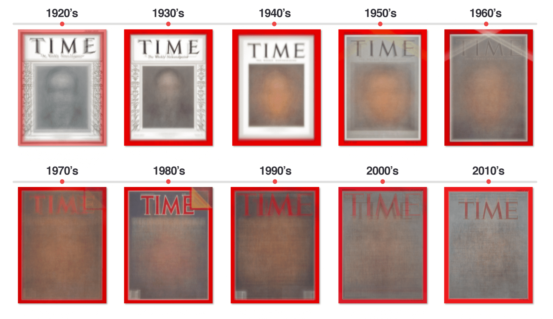
In the remainder of this blog post, we’ll group our Time magazine cover dataset into 10 groups — one group for each of the 10 decades Time magazine has been in publication. Then, for each of these groups, we’ll compute the average of all images in the group, giving us a single visual representation of how the Time cover images looked. This average image will allow us to identify visual trends in the cover images; specifically, marketing and advertising techniques used by Time during a given decade.
Looking for the source code to this post?
Jump right to the downloads section.
Analyzing 91 years of Time magazine covers for visual trends
Before we dive into this post, it might be helpful to read through our previous lesson on scraping Time magazine cover images — reading the previous post is certainly not a requirement, but does help in giving some context.
That said, let’s go ahead and get started. Open up a new file, name it
analyze_covers.py, and let’s get coding:
# import the necessary packages
from __future__ import print_function
import numpy as np
import argparse
import json
import cv2

def filter_by_decade(decade, data):
	# initialize the list of filtered rows
	filtered = []

	# loop over the rows in the data list
	for row in data:
		# grab the publication date of the magazine
		pub = int(row["pubDate"].split("-")[0])

		# if the publication date falls within the current decade,
		# then update the filtered list of data
		if pub >= decade and pub < decade + 10:
			filtered.append(row)

	# return the filtered list of data
	return filtered
Lines 2-6 simply import our necessary packages — nothing too exciting here.
We then define a utility function,
filter_by_decadeon Line 8. As the name suggests, this method will go through our scraped cover images and pull out all covers that fall within a specified decade. Our
filter_by_decadefunction requires two arguments: the
decadewe want to grab cover images for, along with
data, which is simply the
output.jsondata from our previous post.
Now that our method is defined, let’s move on to the body of the function. We’ll initialize
filtered, a list of rows in
datathat match our decade criterion (Line 10).
We then loop over each
rowin the
data(Line 13), extract the publication date (Line 15), and then update our
filteredlist, provided that the publication date falls within our specified
decade(Lines 19 and 20).
Finally, the filtered list of rows is returned to the caller on Line 23.
Now that our helper function is defined, let’s move on to parsing command line arguments and loading our
output.jsonfile:
# import the necessary packages
from __future__ import print_function
import numpy as np
import argparse
import json
import cv2

def filter_by_decade(decade, data):
	# initialize the list of filtered rows
	filtered = []

	# loop over the rows in the data list
	for row in data:
		# grab the publication date of the magazine
		pub = int(row["pubDate"].split("-")[0])

		# if the publication date falls within the current decade,
		# then update the filtered list of data
		if pub >= decade and pub < decade + 10:
			filtered.append(row)

	# return the filtered list of data
	return filtered

# construct the argument parse and parse the arguments
ap = argparse.ArgumentParser()
ap.add_argument("-o", "--output", required=True,
	help="path to output visualizations directory")
args = vars(ap.parse_args())

# load the JSON data file
data = json.loads(open("output.json").read())
Again, here the code is quite simple. Lines 26-29 handle parsing command line arguments. We only need a single switch here,
--visualizations, which is the path to the directory where we will store our average cover images for each decade between 1920 and 2010.
We then load the
output.jsonfile on Line 32 (again, which was generated from our previous post on scraping images with Python + Scrapy).
We are now ready to perform the actual analysis on the Time magazine cover dataset:
# import the necessary packages
from __future__ import print_function
import numpy as np
import argparse
import json
import cv2

def filter_by_decade(decade, data):
	# initialize the list of filtered rows
	filtered = []

	# loop over the rows in the data list
	for row in data:
		# grab the publication date of the magazine
		pub = int(row["pubDate"].split("-")[0])

		# if the publication date falls within the current decade,
		# then update the filtered list of data
		if pub >= decade and pub < decade + 10:
			filtered.append(row)

	# return the filtered list of data
	return filtered

# construct the argument parse and parse the arguments
ap = argparse.ArgumentParser()
ap.add_argument("-o", "--output", required=True,
	help="path to output visualizations directory")
args = vars(ap.parse_args())

# load the JSON data file
data = json.loads(open("output.json").read())

# loop over each individual decade Time magazine has been published
for decade in np.arange(1920, 2020, 10):
	# initialize the magazine covers list
	print("[INFO] processing years: {}-{}".format(decade, decade + 9))
	covers = []

	# loop over the magazine issues belonging to the current decade
	for row in filter_by_decade(decade, data):
		# load the image
		cover = cv2.imread("output/{}".format(row["files"][0]["path"]))

		# if the image is None, then there was an issue loading it
		# (this happens for ~3 images in the dataset, likely due to
		# a download problem during the scraping process)
		if cover is not None:
			# resize the magazine cover, flatten it into a single
			# list, and update the list of covers
			cover = cv2.resize(cover, (400, 527)).flatten()
			covers.append(cover)

	# compute the average image of the covers then write the average
	# image to disk
	avg = np.average(covers, axis=0).reshape((527, 400, 3)).astype("uint8")
	p = "{}/{}.png".format(args["output"], decade)
	cv2.imwrite(p, avg)
We start by looping over each
decadebetween 1920 and 2010 on Line 35 and initialize a list,
covers, to store the actual cover images for the current
decade.
For each of decade, we need to pull out all rows from
output.jsonthat fall within the decade range. Luckily, this is quite easy since we have our
filter_by_decademethod defined above.
The next step is to load the current cover image from disk on Line 43. If the image is
None, then we know there was an issue loading the cover from disk — this happens for about 3 images in the dataset, which is likely due to a download problem or a network issue during the scraping process.
Provided that the
coveris not
None, we we need to resize it to a canonical, known size so we can compute the average of each pixel location (Line 51). Here we resize the image to be a fixed 400 x 527 pixels, ignoring the aspect ratio — the resized image is then flattened into a list of 400 x 527 x 3= 632,400 pixels (the 3 comes from the Red, Green, and Blue channels of the image). If we do not resize the cover to a fixed size, then our rows will not line up and we will be unable to compute the average image for the decade range.
The flattened
coveris then accumulated into the
coverslist on Line 52.
The actual true “analysis” of the decade’s worth of cover images takes place on Line 56 using the
np.averagefunction. Every Time magazine cover image is represented by a flattened row in the
coverslist. Therefore, to compute the average of all covers across a decade, all we need to do is take the mean pixel value of each column. This will leave us with a single list (again, of 632,400-dim), representing the mean value of each Red, Green, and Blue pixel at each (x, y)-coordinate.
However, since the
avgimage is represented as 1D list of floating point values, we cannot visualize it. First, we need to reshape the
avgimage to have a width of 400 pixels, a height of 527 pixels, and a depth of 3 (for each of the Red, Green, and Blue channels, respectively). Finally, since OpenCV expects 8-bit, unsigned integers, we’ll go ahead and convert to
uint8from the
floatdata type returned from
np.average.
Finally, Lines 57 and 58 take our
avgcover image and write it to disk.
To run our script just execute the following command:
$ python analyze_covers.py --output visualizations
After a few seconds, you should see the following images in your
visualizationsdirectory:
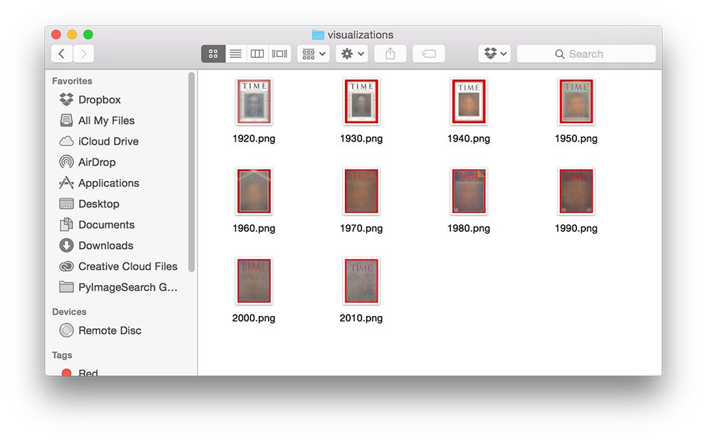
Figure 1: The output of our analyze_covers.py script for image averaging.
Results
Figure 2: Visualizing ten decades’ worth of Time magazine covers.
We now have 10 images in our
visualizationsdirectory, an average each for each of the 10 decades Time magazine has been in publication.
But what do these visualizations actually mean? And what types of insights can we gain from examining them?
As it turns out, quite a lot — especially with respect to how Time performed marketing and advertising with their covers over the past 90+ years:
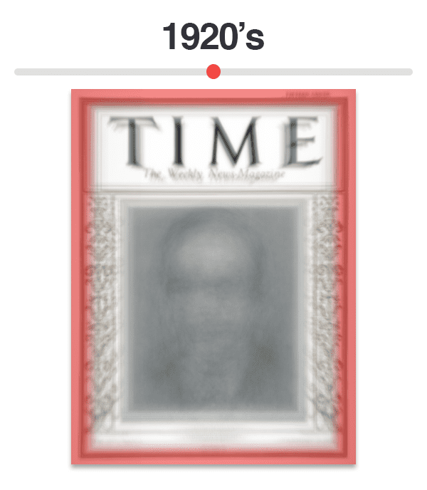
Figure 3: Average of Time magazine covers from 1920-1929.
- Originally, the cover of Time magazine was ALL black and white. But in the late 1920’s the we can see they started to transfer over to the now iconic red border. However, all other aspects of the cover (including the portrait centerpiece) are still in black and white.
- The Time logo always appears at the top of the cover.
- Ornate designs frame the cover portrait on the left and right.
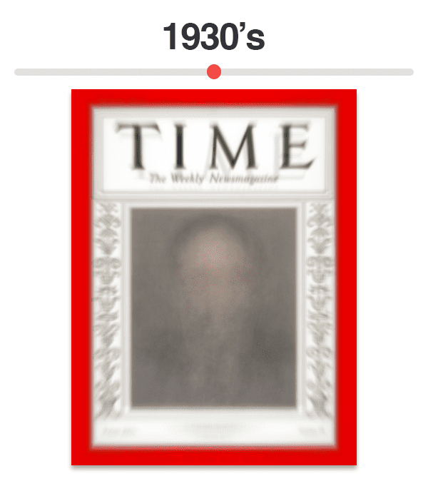
Figure 4: Average of Time magazine covers from 1930-1939.
- Time is now fully committed to their red border, which has actually grown in thickness slightly.
- Overall, not much as changed in the design from the 1920’s to the 1930’s.
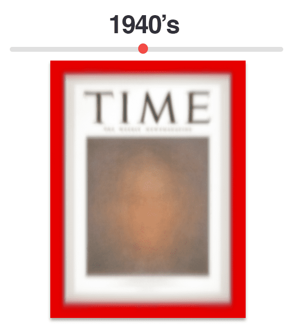
Figure 5: Average of Time magazine covers from 1940-1949.
- The first change we notice is that the red border is not the only color! The portrait of the cover subject is starting to be printed in color. Given that there seems to be a fair amount of color in the portrait region, this change likely took place in the early 1940’s.
- Another subtle alternation is the change in “The Weekly News Magazine” typography directly underneath the “TIME” text.
- It’s also worth noting that the “TIME” text itself is substantially more fixed (i.e. very little variation in placement) as opposed to previous decades.
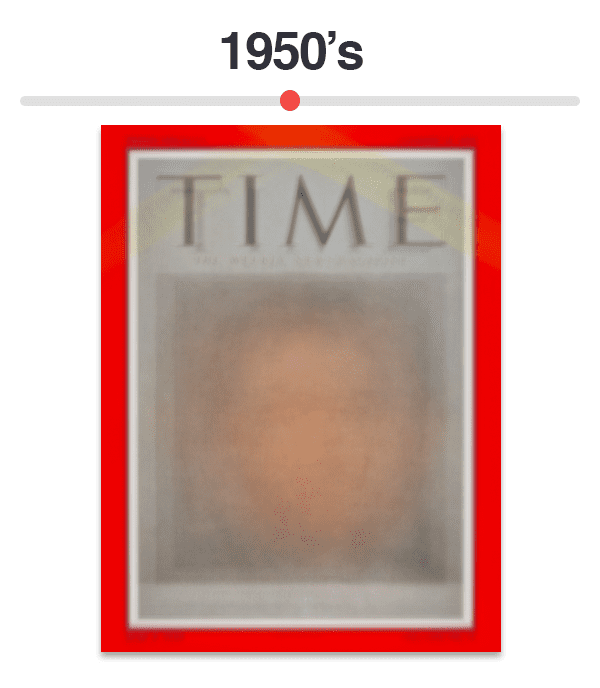
Figure 6: Average of Time magazine covers from 1950-1959.
- The 1950’s cover images demonstrate a dramatic change in Time magazine, both in terms of cover format and marketing and advertising.
- To start, the portrait, once framed by a white border/ornate designs is now expanded to blanket the entire cover — a trend that continues to the modern day.
- Meta-information (such as the name of the issue and publication date) have always been published on the magazine covers; however, we are now starting to see a very fixed and highly formatted version of this meta-information in the four corners of the magazine.
- Most notable is the change in marketing and advertising by using diagonal yellow bars to highlight the cover story of the issue.
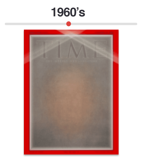
Figure 7: Average of Time magazine covers from 1960-1969.
- The first thing you’ll notice about the 1960’s Time cover is a change in the “TIME” text. While the text appears to be purple, it’s actually a transition from black to red (which averages out to be a purple-ish color). All previous decades of Time used black text for their logo, but in the 1960’s we can see that they converted to their now modern day red.
- Secondly, you’ll see that the “TIME” text is highlighted with a white border which is used to give contrast between the logo and the centerpiece.
- Time is still using diagonal bars for marketing, allowing them to highlight the cover story — but the bars are now more “white” than they are yellow”. The width of the bars has also been slimmed down by 1/3.
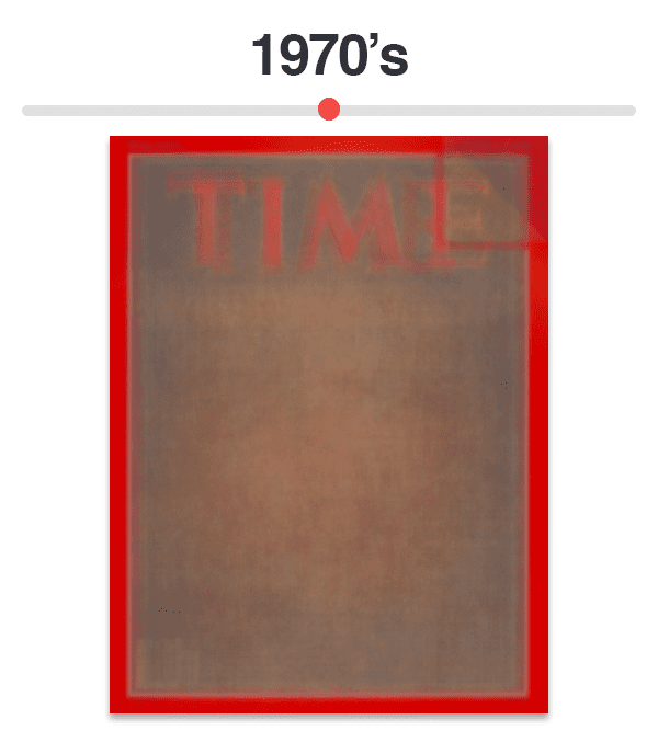
Figure 8: Average of Time magazine covers from 1970-1979.
- Here we see another big change in marketing and advertising strategy — Time is starting to use faux page folds (top-right corner), allowing us to get a “sneak peek” of what’s inside the issue.
- Also note the barcode that is starting to appear in the bottom-left corner of the issue.
- The white border surrounding the “TIME” text has been removed.
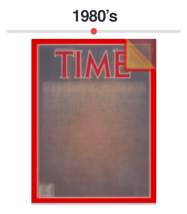
Figure 9: Average of Time magazine covers from 1980-1989.
- The 1980’s issues of Time seem to continue the same faux page fold marketing strategy from the 1970’s.
- They also have re-inserted the white border surrounding the “TIME” text.
- A barcode is now predominately used in the bottom-left corner.
- But also note that a barcode is starting to appear in the bottom-right corner as well.
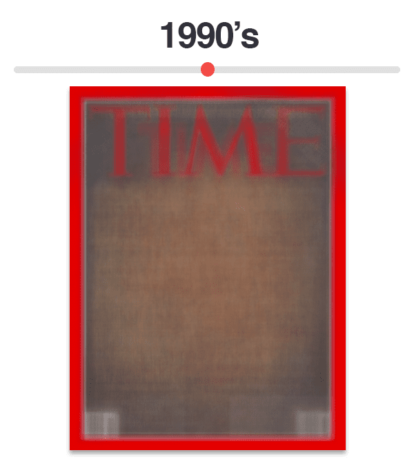
Figure 10: Average of Time magazine covers from 1990-1999.
- Once again, the white border surrounding “TIME” is gone — it makes me curious what types of split tests they were running during these years to figure out if the white border contributed to more sales of the magazine.
- The barcode now consistently appears on the bottom-left and bottom-right corners of the magazine, the choice of barcode placement being highly dependent on aesthetics.
- Also notice that the faux page fold which, which survived nearly two decades, is now gone.
- Lastly, note how the “TIME” logo has become quite variable in size.
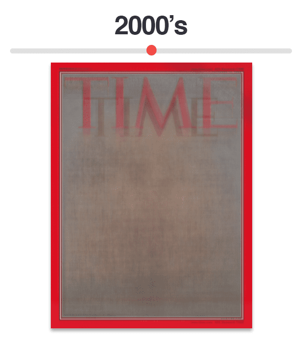
Figure 11: Average of Time magazine covers from 2000-2009.
- The variable logo size has become more pronounced in the 2000’s era.
- We can also see the barcode is completely gone.
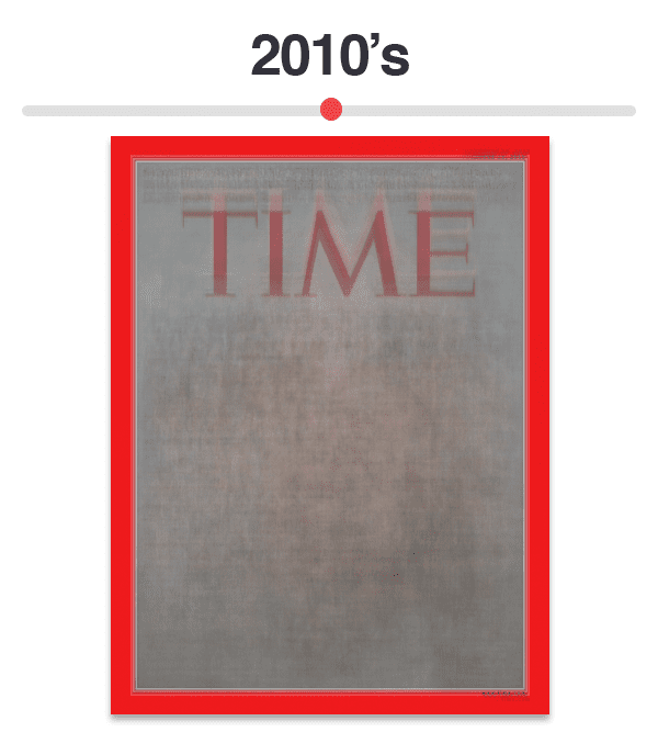
Figure 12: Average of Time magazine covers from 2010-Present.
- We now arrive at the modern day Time magazine cover.
- Overall, there isn’t much difference between the 2010’s and 2000’s.
- However, the size of the Time logo itself seems to be substantially less varied, and only fluctuates along the y-axis.
Summary
In this blog post we explored our Time magazine cover dataset which we gathered in the previous lesson.
To perform a visual analysis of the dataset and identify trends and changes in the magazine covers, we averaged covers together across multiple decades. Given the ten decades Time has been in publication, this left us with ten separate visual representations.
Overall, the changes in covers may seem subtle, but they are actually quite insightful to how the magazine has evolved, specifically in regards to marketing and advertising.
The changes in:
- Logo color and white bordering
- Banners to highlight the cover story
- And faux page folds
Clearly demonstrate that Time magazine was trying to determine which strategies were “eye catching” enough for readers to grab a copy off their local newsstand.
Furthermore, their flip-flopping between white bordering and no white bordering indicates to me that they were performing a series of split tests, accumulating decades worth of data, that eventually resulted in their current, modern day logo.
Downloads:
The post Analyzing 91 years of Time magazine covers for visual trends appeared first on PyImageSearch.