
The watershed algorithm is a classic algorithm used for segmentation and is especially useful when extracting touching or overlapping objects in images, such as the coins in the figure above.
Using traditional image processing methods such as thresholding and contour detection, we would be unable to extract each individual coin from the image — but by leveraging the watershed algorithm, we are able to detect and extract each coin without a problem.
When utilizing the watershed algorithm we must start with user-defined markers. These markers can be either manually defined via point-and-click, or we can automatically or heuristically define them using methods such as thresholding and/or morphological operations.
Based on these markers, the watershed algorithm treats pixels in our input image as local elevation (called a topography) — the method “floods” valleys, starting from the markers and moving outwards, until the valleys of different markers meet each other. In order to obtain an accurate watershed segmentation, the markers must be correctly placed.
In the remainder of this post, I’ll show you how to use the watershed algorithm to segment and extract objects in images that are both touching and overlapping. To accomplish this, we’ll be using a variety of Python packages including SciPy, scikit-image, and OpenCV.
Looking for the source code to this post?
Jump right to the downloads section.
Watershed OpenCV
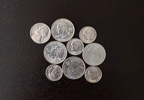
Figure 1: An example image containing touching objects. Our goal is to detect and extract each of these coins individually.
In the above image you can see examples of objects that would be impossible to extract using simple thresholding and contour detection, Since these objects are touching, overlapping, or both, the contour extraction process would treat each group of touching objects as a single object rather than multiple objects.
The problem with basic thresholding and contour extraction
Let’s go ahead and demonstrate a limitation of simple thresholding and contour detection. Open up a new file, name it
contour_only.py, and let’s get coding:
# import the necessary packages
from __future__ import print_function
from skimage.feature import peak_local_max
from skimage.morphology import watershed
from scipy import ndimage
import argparse
import cv2

# construct the argument parse and parse the arguments
ap = argparse.ArgumentParser()
ap.add_argument("-i", "--image", required=True,
	help="path to input image")
args = vars(ap.parse_args())

# load the image and perform pyramid mean shift filtering
# to aid the thresholding step
image = cv2.imread(args["image"])
shifted = cv2.pyrMeanShiftFiltering(image, 21, 51)
cv2.imshow("Input", image)
We start off on Lines 2-7 by importing our necessary packages. Lines 10-13 then parse our command line arguments. We’ll only need a single switch here,
--image, which is the path to the image that we want to process.
From there, we’ll load our image from disk on Line 17, apply pyramid mean shift filtering (Line 18) to help the accuracy of our thresholding step, and finally display our image to our screen. An example of our output thus far can be seen below:
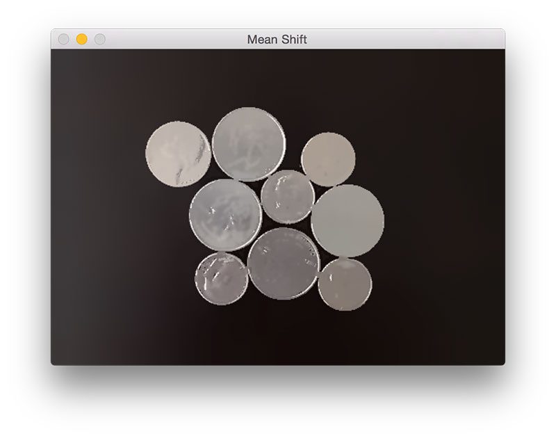
Figure 2: Output from the pyramid mean shift filtering step.
Now, let’s threshold the mean shifted image:
# import the necessary packages
from __future__ import print_function
from skimage.feature import peak_local_max
from skimage.morphology import watershed
from scipy import ndimage
import argparse
import cv2

# construct the argument parse and parse the arguments
ap = argparse.ArgumentParser()
ap.add_argument("-i", "--image", required=True,
	help="path to input image")
args = vars(ap.parse_args())

# load the image and perform pyramid mean shift filtering
# to aid the thresholding step
image = cv2.imread(args["image"])
shifted = cv2.pyrMeanShiftFiltering(image, 21, 51)
cv2.imshow("Input", image)

# convert the mean shift image to grayscale, then apply
# Otsu's thresholding
gray = cv2.cvtColor(shifted, cv2.COLOR_BGR2GRAY)
thresh = cv2.threshold(gray, 0, 255,
	cv2.THRESH_BINARY | cv2.THRESH_OTSU)[1]
cv2.imshow("Thresh", thresh)
Given our input
image, we then convert it to grayscale and apply Otsu’s thresholding to segment the background from the foreground:
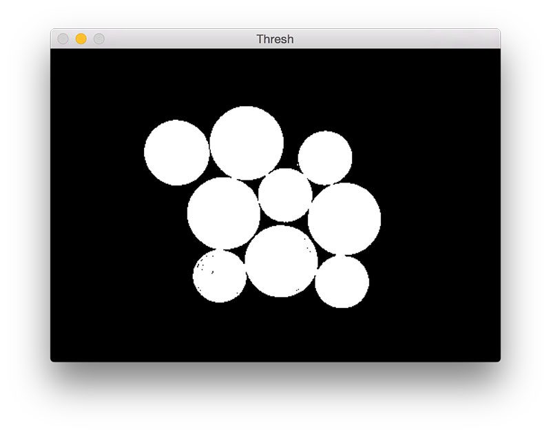
Figure 3: Applying Otsu’s automatic thresholding to segment the foreground coins from the background.
Finally, the last step is to detect contours in the thresholded image and draw each individual contour:
# import the necessary packages
from __future__ import print_function
from skimage.feature import peak_local_max
from skimage.morphology import watershed
from scipy import ndimage
import argparse
import cv2

# construct the argument parse and parse the arguments
ap = argparse.ArgumentParser()
ap.add_argument("-i", "--image", required=True,
	help="path to input image")
args = vars(ap.parse_args())

# load the image and perform pyramid mean shift filtering
# to aid the thresholding step
image = cv2.imread(args["image"])
shifted = cv2.pyrMeanShiftFiltering(image, 21, 51)
cv2.imshow("Input", image)

# convert the mean shift image to grayscale, then apply
# Otsu's thresholding
gray = cv2.cvtColor(shifted, cv2.COLOR_BGR2GRAY)
thresh = cv2.threshold(gray, 0, 255,
	cv2.THRESH_BINARY | cv2.THRESH_OTSU)[1]
cv2.imshow("Thresh", thresh)

# find contours in the thresholded image
cnts = cv2.findContours(thresh.copy(), cv2.RETR_EXTERNAL,
	cv2.CHAIN_APPROX_SIMPLE)[-2]
print("[INFO] {} unique contours found".format(len(cnts)))

# loop over the contours
for (i, c) in enumerate(cnts):
	# draw the contour
	((x, y), _) = cv2.minEnclosingCircle(c)
	cv2.putText(image, "#{}".format(i + 1), (int(x) - 10, int(y)),
		cv2.FONT_HERSHEY_SIMPLEX, 0.6, (0, 0, 255), 2)
	cv2.drawContours(image, [c], -1, (0, 255, 0), 2)

# show the output image
cv2.imshow("Image", image)
cv2.waitKey(0)
Below we can see the output of our image processing pipeline:
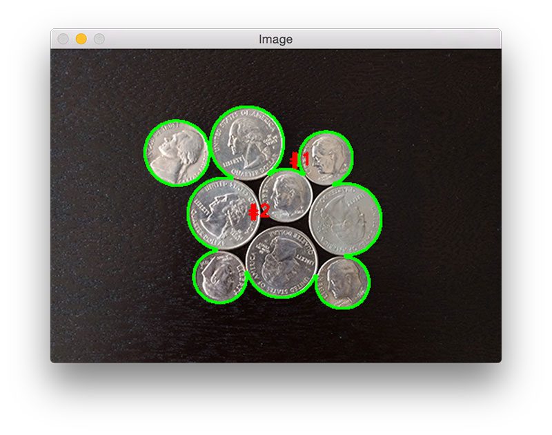
Figure 4: The output of our simple image processing pipeline. Unfortunately, our results are pretty poor — we are not able to detect each individual coin.
As you can see, our results are pretty terrible. Using simple thresholding and contour detection our Python script reports that there are only two coins in the images, even though there are clearly nine of them.
The reason for this problem arises from the fact that coin borders are touching each other in the image — thus, the
cv2.findContoursfunction only sees the coin groups as a single object when in fact they are multiple, separate coins.
Note: A series of morphological operations (specifically, erosions) would help us for this particular image. However, for objects that are overlapping these erosions would not be sufficient. For the sake of this example, let’s pretend that morphological operations are not a viable option so that we may explore the watershed algorithm.
Using the watershed algorithm for segmentation
Now that we understand the limitations of simple thresholding and contour detection, let’s move on to the watershed algorithm. Open up a new file, name it
watershed.py, and insert the following code:
# import the necessary packages
from skimage.feature import peak_local_max
from skimage.morphology import watershed
from scipy import ndimage
import numpy as np
import argparse
import cv2

# construct the argument parse and parse the arguments
ap = argparse.ArgumentParser()
ap.add_argument("-i", "--image", required=True,
	help="path to input image")
args = vars(ap.parse_args())

# load the image and perform pyramid mean shift filtering
# to aid the thresholding step
image = cv2.imread(args["image"])
shifted = cv2.pyrMeanShiftFiltering(image, 21, 51)
cv2.imshow("Input", image)

# convert the mean shift image to grayscale, then apply
# Otsu's thresholding
gray = cv2.cvtColor(shifted, cv2.COLOR_BGR2GRAY)
thresh = cv2.threshold(gray, 0, 255,
	cv2.THRESH_BINARY | cv2.THRESH_OTSU)[1]
cv2.imshow("Thresh", thresh)
Again, we’ll start on Lines 2-7 by importing our required packages. We’ll be using functions from SciPy, scikit-image, and OpenCV. If you don’t already have SciPy and scikit-image installed on your system, you can use
pipto install them for you:
$ pip install scipy
$ pip install -U scikit-image
Lines 10-13 handle parsing our command line arguments. Just like in the previous example, we only need a single switch, the path to the image
--imagewe are going to apply the watershed algorithm to.
From there, Lines 17 and 18 load our image from disk and apply pyramid mean shift filtering. Lines 23-25 perform grayscale conversion and thresholding.
Given our thresholded image, we can now apply the watershed algorithm:
# import the necessary packages
from skimage.feature import peak_local_max
from skimage.morphology import watershed
from scipy import ndimage
import numpy as np
import argparse
import cv2

# construct the argument parse and parse the arguments
ap = argparse.ArgumentParser()
ap.add_argument("-i", "--image", required=True,
	help="path to input image")
args = vars(ap.parse_args())

# load the image and perform pyramid mean shift filtering
# to aid the thresholding step
image = cv2.imread(args["image"])
shifted = cv2.pyrMeanShiftFiltering(image, 21, 51)
cv2.imshow("Input", image)

# convert the mean shift image to grayscale, then apply
# Otsu's thresholding
gray = cv2.cvtColor(shifted, cv2.COLOR_BGR2GRAY)
thresh = cv2.threshold(gray, 0, 255,
	cv2.THRESH_BINARY | cv2.THRESH_OTSU)[1]
cv2.imshow("Thresh", thresh)

# compute the exact Euclidean distance from every binary
# pixel to the nearest zero pixel, then find peaks in this
# distance map
D = ndimage.distance_transform_edt(thresh)
localMax = peak_local_max(D, indices=False, min_distance=20,
	labels=thresh)

# perform a connected component analysis on the local peaks,
# using 8-connectivity, then appy the Watershed algorithm
markers = ndimage.label(localMax, structure=np.ones((3, 3)))[0]
labels = watershed(-D, markers, mask=thresh)
print("[INFO] {} unique segments found".format(len(np.unique(labels)) - 1))
The first step in applying the watershed algorithm for segmentation is to compute the Euclidean Distance Transform (EDT) via the
distance_transform_edtfunction (Line 31). As the name suggests, this function computes the Euclidean distance to the closest zero (i.e., background pixel) for each of the foreground pixels. We can visualize the EDT in the figure below:
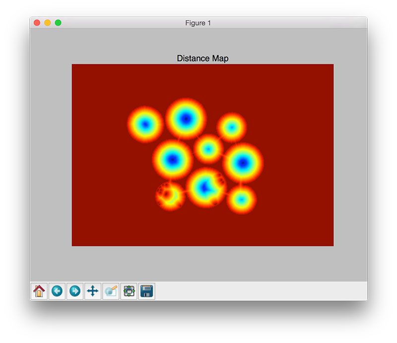
Figure 5: Visualizing the Euclidean Distance Transform.
On Line 32 we take
D, our distance map, and find peaks (i.e., local maxima) in the map. We’ll ensure that is at least a 20 pixel distance between each peak.
Line 37 takes the output of the
peak_local_maxfunction and applies a connected-component analysis using 8-connectivity. The output of this function gives us our
markerswhich we then feed into the
watershedfunction on Line 38. Since the watershed algorithm assumes our markers represent local minima (i.e., valleys) in our distance map, we take the negative value of
D.
The
watershedfunction returns a matrix of
labels, a NumPy array with the same width and height as our input image. Each pixel value as a unique label value. Pixels that have the same label value belong to the same object.
The last step is to simply loop over the unique label values and extract each of the unique objects:
# import the necessary packages
from skimage.feature import peak_local_max
from skimage.morphology import watershed
from scipy import ndimage
import numpy as np
import argparse
import cv2

# construct the argument parse and parse the arguments
ap = argparse.ArgumentParser()
ap.add_argument("-i", "--image", required=True,
	help="path to input image")
args = vars(ap.parse_args())

# load the image and perform pyramid mean shift filtering
# to aid the thresholding step
image = cv2.imread(args["image"])
shifted = cv2.pyrMeanShiftFiltering(image, 21, 51)
cv2.imshow("Input", image)

# convert the mean shift image to grayscale, then apply
# Otsu's thresholding
gray = cv2.cvtColor(shifted, cv2.COLOR_BGR2GRAY)
thresh = cv2.threshold(gray, 0, 255,
	cv2.THRESH_BINARY | cv2.THRESH_OTSU)[1]
cv2.imshow("Thresh", thresh)

# compute the exact Euclidean distance from every binary
# pixel to the nearest zero pixel, then find peaks in this
# distance map
D = ndimage.distance_transform_edt(thresh)
localMax = peak_local_max(D, indices=False, min_distance=20,
	labels=thresh)

# perform a connected component analysis on the local peaks,
# using 8-connectivity, then appy the Watershed algorithm
markers = ndimage.label(localMax, structure=np.ones((3, 3)))[0]
labels = watershed(-D, markers, mask=thresh)
print("[INFO] {} unique segments found".format(len(np.unique(labels)) - 1))

# loop over the unique labels returned by the Watershed
# algorithm
for label in np.unique(labels):
	# if the label is zero, we are examining the 'background'
	# so simply ignore it
	if label == 0:
		continue

	# otherwise, allocate memory for the label region and draw
	# it on the mask
	mask = np.zeros(gray.shape, dtype="uint8")
	mask[labels == label] = 255

	# detect contours in the mask and grab the largest one
	cnts = cv2.findContours(mask.copy(), cv2.RETR_EXTERNAL,
		cv2.CHAIN_APPROX_SIMPLE)[-2]
	c = max(cnts, key=cv2.contourArea)

	# draw a circle enclosing the object
	((x, y), r) = cv2.minEnclosingCircle(c)
	cv2.circle(image, (int(x), int(y)), int(r), (0, 255, 0), 2)
	cv2.putText(image, "#{}".format(label), (int(x) - 10, int(y)),
		cv2.FONT_HERSHEY_SIMPLEX, 0.6, (0, 0, 255), 2)

# show the output image
cv2.imshow("Output", image)
cv2.waitKey(0)
On Line 43 we start looping over each of the unique
labels. If the
labelis zero, then we are examining the “background component”, so we simply ignore it.
Otherwise, Lines 51 and 52 allocate memory for our
maskand set the pixels belonging to the current label to 255 (white). We can see an example of such a mask below on the right:

Figure 6: An example mask where we are detecting and extracting only a single object from the image.
On Lines 55-57 we detect contours in the
maskand extract the largest one — this contour will represent the outline/boundary of a given object in the image.
Finally, given the contour of the object, all we need to do is draw the enclosing circle boundary surrounding the object on Lines 60-63. We could also compute the bounding box of the object, apply a bitwise operation, and extract each individual object as well.
Finally, Lines 66 and 67 display the output image to our screen:
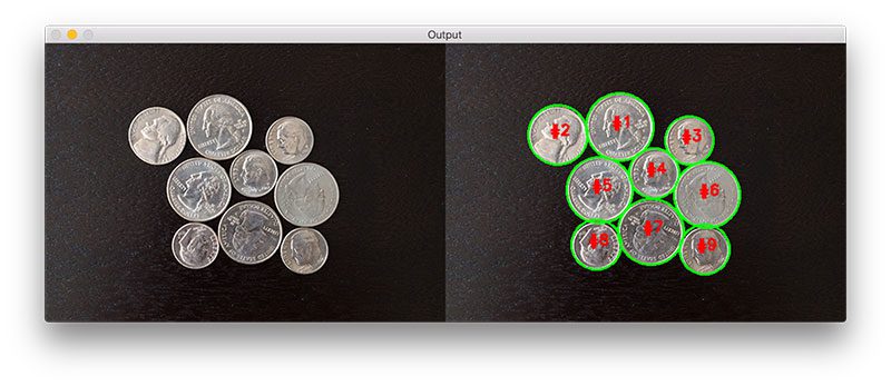
Figure 7: The final output of our watershed algorithm — we have been able to cleanly detect and draw the boundaries of each coin in the image, even though their edges are touching.
As you can see, we have successfully detected all nine coins in the image. Furthermore, we have been able to cleanly draw the boundaries surrounding each coin as well. This is in stark contrast to the previous example using simple thresholding and contour detection where only two objects were (incorrectly) detected.
Applying the watershed algorithm to images
Now that our
watershed.pyscript is finished up, let’s apply it to a few more images and investigate the results:
$ python watershed.py --image images/coins_02.png
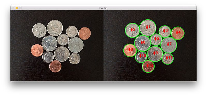
Figure 8: Again, we are able to cleanly segment each of the coins in the image.
Let’s try another image, this time with overlapping coins:
$ python watershed.py --image images/coins_03.png
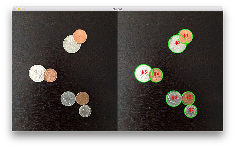
Figure 9: The watershed algorithm is able to segment the overlapping coins from each other.
In the following image, I decided to apply the watershed algorithm to the task of pill counting:
$ python watershed.py --image images/pills_01.png
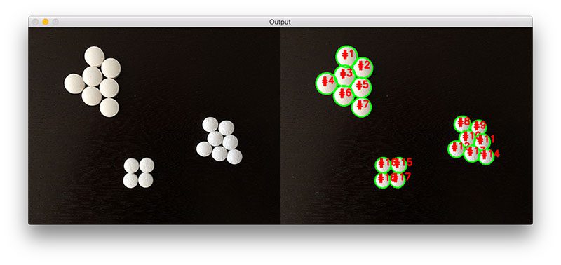
Figure 10: We are able to correctly count the number of pills in the image.
The same is true for this image as well:
$ python watershed.py --image images/pills_02.png
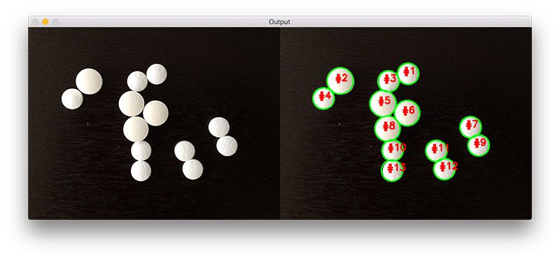
Figure 11: Applying the watershed algorithm with OpenCV to count the number of pills in an image.
Summary
In this blog post we learned how to apply the watershed algorithm, a classic segmentation algorithm used to detect and extract objects in images that are touching and/or overlapping.
To apply the watershed algorithm we need to define markers which correspond to the objects in our image. These markers can be either user-defined or we can apply image processing techniques (such as thresholding) to find the markers for us. When applying the watershed algorithm, it’s absolutely critical that we obtain accurate markers.
Given our markers, we can compute the Euclidean Distance Transform and pass the distance map to the watershed function itself, which “floods” valleys in the distance map, starting from the initial markers and moving outwards. Where the “pools” of water meet can be considered boundary lines in the segmentation process.
The output of the watershed algorithm is a set of labels, where each label corresponds to a unique object in the image. From there, all we need to do is loop over each of the labels individually and extract each object.
Anyway, I hope you enjoyed this post! Be sure download the code and give it a try. Try playing with various parameters, specifically the
min_distanceargument to the
peak_local_maxfunction. Note how varying the value of this parameter can change the output image.
Downloads:
The post Watershed OpenCV appeared first on PyImageSearch.