In this tutorial, you will learn how to train your own custom dlib shape predictor. You’ll then learn how to take your trained dlib shape predictor and use it to predict landmarks on input images and real-time video streams.

Today kicks off a brand new two-part series on training custom shape predictors with dlib:

1. Part #1: Training a custom dlib shape predictor (today’s tutorial)
2. Part #2: Tuning dlib shape predictor hyperparameters to balance speed, accuracy, and model size (next week’s tutorial)

Shape predictors, also called landmark predictors, are used to predict key (x, y)-coordinates of a given “shape”.

The most common, well-known shape predictor is dlib’s facial landmark predictor used to localize individual facial structures, including the:

• Eyes
• Eyebrows
• Nose
• Lips/mouth
• Jawline

Facial landmarks are used for face alignment (a method to improve face recognition accuracy), building a “drowsiness detector” to detect tired, sleepy drivers behind the wheel, face swapping, virtual makeover applications, and much more.

However, just because facial landmarks are the most popular type of shape predictor, doesn’t mean we can’t train a shape predictor to localize other shapes in an image!

For example, you could use a shape predictor to:

• Automatically localize the four corners of a piece of paper when building a computer vision-based document scanner.
• Detect the key, structural joints of the human body (feet, knees, elbows, etc.).
• Localize the tips of your fingers when building an AR/VR application.

Today we’ll be exploring shape predictors in more detail, including how you can train your own custom shape predictor using the dlib library.

To learn how to train your own dlib shape predictor, just keep reading!

Tuning a custom dlib shape predictor

In the first part of this tutorial, we’ll briefly discuss what shape/landmark predictors are and how they can be used to predict specific locations on structural objects.

From there we’ll review the iBUG 300-W dataset, a common dataset used to train shape predictors used to localize specific locations on the human face (i.e., facial landmarks).

I’ll then show you how to train your own custom dlib shape predictor, resulting in a model that can balance speed, accuracy, and model size.

Finally, we’ll put our shape predictor to the test and apply it to a set of input images/video streams, demonstrating that our shape predictor is capable of running in real-time.

We’ll wrap up the tutorial with a discussion of next steps.

What are shape/landmark predictors?

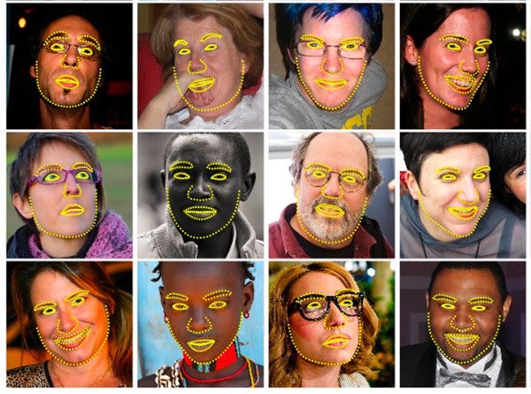
Figure 1: Training a custom dlib shape predictor on facial landmarks (image source).

Shape/landmark predictors are used to localize specific (x, y)-coordinates on an input “shape”. The term “shape” is is arbitrary, but it’s assumed that the shape is structural in nature.

Examples of structural shapes include:

• Faces
• Hands
• Fingers
• Toes
• etc.

For example, faces come in all different shapes and sizes, and they all share common structural characteristics — the eyes are above the nose, the nose is above the mouth, etc.

The goal of shape/landmark predictors is to exploit this structural knowledgem and given enough training data, learn how to automatically predict the location of these structures.

How do shape/landmark predictors work?

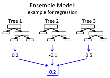
Figure 2: How do shape/landmark predictors work? The dlib library implements a shape predictor algorithm with an ensemble of regression tress approach using the method described by Kazemi and Sullivan in their 2014 CVPR paper (image source).

There are a variety of shape predictor algorithms. Exactly which one you use depends on whether:

• You’re working with 2D or 3D data
• You need to utilize deep learning
• Or, if traditional Computer Vision and Machine Learning algorithms will suffice

The shape predictor algorithm implemented in the dlib library comes from Kazemi and Sullivan 2014 CVPR paper, One Millisecond Face Alignment with an Ensemble of Regression Trees.

To estimate the landmark locations, the algorithm:

• Examines a sparse set of input pixel intensities (i.e., the “features” to the input model)
• Passes the features into an Ensemble of Regression Trees (ERT)
• Refines the predicted locations to improve accuracy through a cascade of regressors

The end result is a shape predictor that can run in super real-time!

For more details on the inner-workings of the landmark prediction, be sure to refer to Kazemi and Sullivan’s 2014 publication.

The iBUG 300-W dataset

Figure 3: In this tutorial we will use the iBUG 300-W face landmark dataset to learn how to train a custom dlib shape predictor.

To train our custom dlib shape predictor, we’ll be utilizing the iBUG 300-W dataset (but with a twist).

The goal of iBUG-300W is to train a shape predictor capable of localizing each individual facial structure, including the eyes, eyebrows, nose, mouth, and jawline.

The dataset itself consists of 68 pairs of integer values — these values are the (x, y)-coordinates of the facial structures are depicted in Figure 2 above.

To create the iBUG-300W dataset, researchers manually and painstakingly annotated and labeled each of the 68 coordinates on a total of 7,764 images.

A model trained on iBUG-300W can predict the location of each of these 68 (x, y)-coordinate pairs and can, therefore, localize each of the locations on the face.

That’s all fine and good…

…but what if wanted to train a shape predictor to localize just the eyes?

How might we go about doing that?

Balancing shape predictor model speed and accuracy

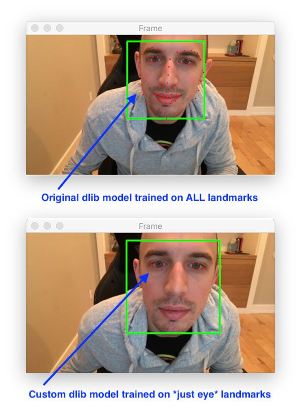
Figure 4: We will train a custom dlib shape/landmark predictor to recognize just eyes in this tutorial.

Let’s suppose for a second that you want to train a custom shape predictor to localize just the location of the eyes.

We would have two options to accomplish this task:

1. Utilize dlib’s pre-trained facial landmark detector used to localize all facial structures and then discard all localizations except for the eyes.
2. Train our own custom dlib landmark predictor that returns just the locations of the eyes.

In some cases you may be able to get away with the first option; however, there are two problems there, namely regarding your model speed and your model size.

Model speed: Even though you’re only interested in a subset of the landmark predictions, your model is still responsible for predicting the entire set of landmarks. You can’t just tell your model “Oh hey, just give me those locations, don’t bother computing the rest.” It doesn’t work like that — it’s an “all or nothing” calculation.

Model size: Since your model needs to know how to predict all landmark locations it was trained on, it therefore needs to store quantified information on how to predict each of these locations. The more information it needs to store, the larger your model size is.

Think of your shape predictor model size as a grocery list — out of a list of 20 items, you may only truly need eggs and a gallon of milk, but if you’re heading to the store, you’re going to be purchasing all the items on that list because that’s what your family expects you to do!

The model size is the same way.

Your model doesn’t “care” that you only truly “need” a subset of the landmark predictions; it was trained to predict all of them so you’re going to get all of them in return!

If you only need a subset of specific landmarks you should consider training your own custom shape predictor — you’ll end up with a model that is both smaller and faster.

In the context of today’s tutorial, we’ll be training a custom dlib shape predictor to localize just the eye locations from the iBUG 300-W dataset.

Such a model could be utilized in a virtual makeover application used to apply just eyeliner/mascara or it could be used in a drowsiness detector used to detect tired drivers behind the wheel of a car.

Configuring your dlib development environment

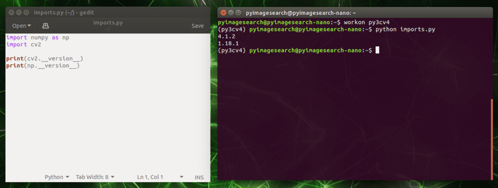
To follow along with today’s tutorial, you will need a virtual environment with the following packages installed:

• dlib
• OpenCV
• imutils

Luckily, each of these packages is pip-installable, but there are a handful of pre-requisites including virtual environments. Be sure to follow these two guides for additional information:

• Install dlib (the easy, complete guide)
• pip install opencv

The pip install commands include:

$ workon <env-name>
$ pip install dlib
$ pip install opencv-contrib-python
$ pip install imutils

The

workon

virtualenv

virtualenvwrapper

Downloading the iBUG 300-W dataset

Before we get too far into this tutorial, take a second now to download the iBUG 300-W dataset (~1.7GB):

http://dlib.net/files/data/ibug_300W_large_face_landmark_dataset.tar.gz

You’ll also want to use the “Downloads” section of this blog post to download the source code.

I recommend placing the iBug 300W dataset into the zip associated with the download of this tutorial like this:

$ unzip custom-dlib-shape-predictor.zip
...
$ cd custom-dlib-shape-predictor
$ mv ~/Downloads/ibug_300W_large_face_landmark_dataset.tar.gz .
$ tar -xvf ibug_300W_large_face_landmark_dataset.tar.gz
...

Alternatively (i.e. rather than clicking the hyperlink above), use

wget

$ unzip custom-dlib-shape-predictor.zip
...
$ cd custom-dlib-shape-predictor
$ wget http://dlib.net/files/data/ibug_300W_large_face_landmark_dataset.tar.gz
$ tar -xvf ibug_300W_large_face_landmark_dataset.tar.gz
...

From there you can follow along with the rest of the tutorial.

Project Structure

Assuming you have followed the instructions in the previous section, your project directory is now organized as follows:

$ tree --dirsfirst --filelimit 10
.
├── ibug_300W_large_face_landmark_dataset
│   ├── afw [1011 entries]
│   ├── helen
│   │   ├── testset [990 entries]
│   │   └── trainset [6000 entries]
│   ├── ibug [405 entries]
│   ├── image_metadata_stylesheet.xsl
│   ├── labels_ibug_300W.xml
│   ├── labels_ibug_300W_test.xml
│   ├── labels_ibug_300W_train.xml
│   └── lfpw
│       ├── testset [672 entries]
│       └── trainset [2433 entries]
├── ibug_300W_large_face_landmark_dataset.tar.gz
├── eye_predictor.dat
├── parse_xml.py
├── train_shape_predictor.py
├── evaluate_shape_predictor.py
└── predict_eyes.py

9 directories, 10 files

The iBug 300-W dataset is extracted in the

ibug_300W_large_face_landmark_dataset/

1. parse_xml.py

   : Parses the train/test XML dataset files for eyes-only landmark coordinates.

2. train_shape_predictor.py

    : Accepts the parsed XML files to train our shape predictor with dlib.

3. evaluate_shape_predictor.py

   : Calculates the Mean Average Error (MAE) of our custom shape predictor.

4. predict_eyes.py

   : Performs shape prediction using our custom dlib shape predictor, trained to only recognize eye landmarks.

We’ll begin by inspecting our input XML files in the next section.

Understanding the iBUG-300W XML file structure

We’ll be using the iBUG-300W to train our shape predictor; however, we have a bit of a problem:

iBUG-300W supplies (x, y)-coordinate pairs for all facial structures in the dataset (i.e., eyebrows, eyes, nose, mouth, and jawline)…

…however, we want to train our shape predictor on just the eyes!

So, what are we going to do?

Are we going to find another dataset that doesn’t include the facial structures we don’t care about?

Manually open up the training file and delete the coordinate pairs for the facial structures we don’t need?

Simply give up, take our ball, and go home?

Of course not!

We’re programmers and engineers — all we need is some basic file parsing to create a new training file that includes just the eye coordinates.

To understand how we can do that, let’s first consider how facial landmarks are annotated in the iBUG-300W dataset by examining the

labels_ibug_300W_train.xml

...
<images>
  <image file='lfpw/trainset/image_0457.png'>
    <box top='78' left='74' width='138' height='140'>
      <part name='00' x='55' y='141'/>
      <part name='01' x='59' y='161'/>
      <part name='02' x='66' y='182'/>
      <part name='03' x='75' y='197'/>
      <part name='04' x='90' y='209'/>
      <part name='05' x='108' y='220'/>
      <part name='06' x='131' y='226'/>
      <part name='07' x='149' y='232'/>
      <part name='08' x='167' y='230'/>
      <part name='09' x='181' y='225'/>
      <part name='10' x='184' y='208'/>
      <part name='11' x='186' y='193'/>
      <part name='12' x='185' y='179'/>
      <part name='13' x='184' y='167'/>
      <part name='14' x='186' y='152'/>
      <part name='15' x='185' y='142'/>
      <part name='16' x='181' y='133'/>
      <part name='17' x='95' y='128'/>
      <part name='18' x='105' y='121'/>
      <part name='19' x='117' y='117'/>
      <part name='20' x='128' y='115'/>
      <part name='21' x='141' y='116'/>
      <part name='22' x='156' y='115'/>
      <part name='23' x='162' y='110'/>
      <part name='24' x='169' y='108'/>
      <part name='25' x='175' y='108'/>
      <part name='26' x='180' y='109'/>
      <part name='27' x='152' y='127'/>
      <part name='28' x='157' y='136'/>
      <part name='29' x='162' y='145'/>
      <part name='30' x='168' y='154'/>
      <part name='31' x='152' y='166'/>
      <part name='32' x='158' y='166'/>
      <part name='33' x='163' y='168'/>
      <part name='34' x='167' y='166'/>
      <part name='35' x='171' y='164'/>
      <part name='36' x='111' y='134'/>
      <part name='37' x='116' y='130'/>
      <part name='38' x='124' y='128'/>
      <part name='39' x='129' y='130'/>
      <part name='40' x='125' y='134'/>
      <part name='41' x='118' y='136'/>
      <part name='42' x='161' y='127'/>
      <part name='43' x='166' y='123'/>
      <part name='44' x='173' y='122'/>
      <part name='45' x='176' y='125'/>
      <part name='46' x='173' y='129'/>
      <part name='47' x='167' y='129'/>
      <part name='48' x='139' y='194'/>
      <part name='49' x='151' y='186'/>
      <part name='50' x='159' y='180'/>
      <part name='51' x='163' y='182'/>
      <part name='52' x='168' y='180'/>
      <part name='53' x='173' y='183'/>
      <part name='54' x='176' y='189'/>
      <part name='55' x='174' y='193'/>
      <part name='56' x='170' y='197'/>
      <part name='57' x='165' y='199'/>
      <part name='58' x='160' y='199'/>
      <part name='59' x='152' y='198'/>
      <part name='60' x='143' y='194'/>
      <part name='61' x='159' y='186'/>
      <part name='62' x='163' y='187'/>
      <part name='63' x='168' y='186'/>
      <part name='64' x='174' y='189'/>
      <part name='65' x='168' y='191'/>
      <part name='66' x='164' y='192'/>
      <part name='67' x='160' y='192'/>
    </box>
  </image>
...

All training data in the iBUG-300W dataset is represented by a structured XML file.

Each image has an

image

Inside the

image

file

Additionally, each

image

box

The

box

box

1. top

   : The starting y-coordinate of the bounding box.

2. left

   : The starting x-coordinate of the bounding box.

3. width

   : The width of the bounding box.

4. height

   : The height of the bounding box.

Inside the

box

part

part

Notice that each

part

1. name

   : The index/name of the specific facial landmark.

2. x

   : The x-coordinate of the landmark.

3. y

   : The y-coordinate of the landmark.

So, how do these landmarks map to specific facial structures?

The answer lies in the following figure:

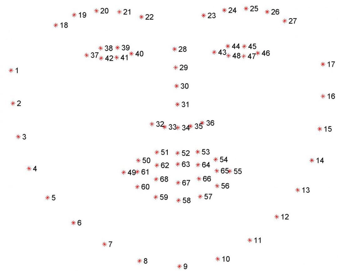
Figure 5: Visualizing the 68 facial landmark coordinates from the iBUG 300-W dataset.

The coordinates in Figure 5 are 1-indexed so to map the coordinate

name

Based on the visualization, we can then derive which

name

• The mouth can be accessed through points [48, 68].
• The right eyebrow through points [17, 22].
• The left eyebrow through points [22, 27].
• The right eye using [36, 42].
• The left eye with [42, 48].
• The nose using [27, 35].
• And the jaw via [0, 17].

Since we’re only interested in the eyes, we therefore need to parse out points [36, 48), again keeping in mind that:

• Our coordinates are zero-indexed in the XML file
• And the closing parenthesis “)” in [36, 48) is mathematical notation implying “non-inclusive”.

Now that we understand the structure of the iBUG-300W training file, we can move on to parsing out only the eye coordinates.

Building an “eyes only” shape predictor dataset

Let’s create a Python script to parse the iBUG-300W XML files and extract only the eye coordinates (which we’ll then train a custom dlib shape predictor on in the following section).

Open up the

parse_xml.py

# import the necessary packages
import argparse
import re

# construct the argument parser and parse the arguments
ap = argparse.ArgumentParser()
ap.add_argument("-i", "--input", required=True,
	help="path to iBug 300-W data split XML file")
ap.add_argument("-t", "--output", required=True,
	help="path output data split XML file")
args = vars(ap.parse_args())

Lines 2 and 3 import necessary packages.

We’ll use two of Python’s built-in modules: (1)

argparse

re

Our script requires two command line arguments:

• --input

  : The path to our input data split XML file (i.e. from the iBug 300-W dataset).

• --output

  : The path to our output eyes-only output XML file.

Let’s go ahead and define the indices of our eye coordinates:

# in the iBUG 300-W dataset, each (x, y)-coordinate maps to a specific
# facial feature (i.e., eye, mouth, nose, etc.) -- in order to train a
# dlib shape predictor on *just* the eyes, we must first define the
# integer indexes that belong to the eyes
LANDMARKS = set(list(range(36, 48)))

Our eye landmarks are specified on Line 17. Refer to Figure 5, keeping in mind that the figure is 1-indexed while Python is 0-indexed.

We’ll be training our custom shape predictor on eye locations; however, you could just as easily train an eyebrow, nose, mouth, or jawline predictor, including any combination or subset of these structures, by modifying the

LANDMARKS

Now let’s define our regular expression and load the original input XML file:

# to easily parse out the eye locations from the XML file we can
# utilize regular expressions to determine if there is a 'part'
# element on any given line
PART = re.compile("part name='[0-9]+'")

# load the contents of the original XML file and open the output file
# for writing
print("[INFO] parsing data split XML file...")
rows = open(args["input"]).read().strip().split("\n")
output = open(args["output"], "w")

Our regular expression on Line 22 will soon enable extracting

part

Line 27 loads the contents of input XML file.

Line 28 opens our output XML file for writing.

Now we’re ready to loop over the input XML file to find and extract the eye landmarks:

# loop over the rows of the data split file
for row in rows:
	# check to see if the current line has the (x, y)-coordinates for
	# the facial landmarks we are interested in
	parts = re.findall(PART, row)

	# if there is no information related to the (x, y)-coordinates of
	# the facial landmarks, we can write the current line out to disk
	# with no further modifications
	if len(parts) == 0:
		output.write("{}\n".format(row))

	# otherwise, there is annotation information that we must process
	else:
		# parse out the name of the attribute from the row
		attr = "name='"
		i = row.find(attr)
		j = row.find("'", i + len(attr) + 1)
		name = int(row[i + len(attr):j])

		# if the facial landmark name exists within the range of our
		# indexes, write it to our output file
		if name in LANDMARKS:
			output.write("{}\n".format(row))

# close the output file
output.close()

Line 31 begins a loop over the

rows

• Determine if the current

  row

  contains a

  part

  element via regular expression matching (Line 34).
  • If it does not contain a

    part

    element, write the row back out to file (Lines 39 and 40).
  • If it does contain a

    part

    element, we need to parse it further (Lines 43-53).
    • Here we extract

      name

      attribute from the

      part

      .
    • And then check to see if the

      name

      exists in the

      LANDMARKS

      we want to train a shape predictor to localize. If so, we write the

      row

      back out to disk (otherwise we ignore the particular

      name

      as it’s not a landmark we want to localize).
• Wrap up the script by closing our

  output

  XML file (Line 56).

Note: Most of our

parse_xml.py

Creating our training and testing splits

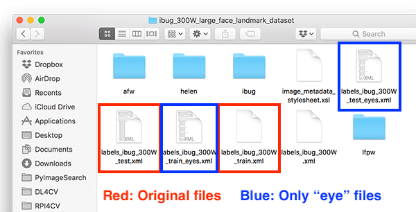
Figure 6: Creating our “eye only” face landmark training/testing XML files for training a dlib custom shape predictor with Python.

At this point in the tutorial I assume you have both:

1. Downloaded the iBUG-300W dataset from the “Downloading the iBUG 300-W dataset” section above
2. Used the “Downloads” section of this tutorial to download the source code.

You can use the following command to generate our new training file by parsing only the eye landmark coordinates from the original training file:

$ python parse_xml.py \
	--input ibug_300W_large_face_landmark_dataset/labels_ibug_300W_train.xml \
	--output ibug_300W_large_face_landmark_dataset/labels_ibug_300W_train_eyes.xml
[INFO] parsing data split XML file...

Similarly, you can do the same to create our new testing file:

$ python parse_xml.py \
	--input ibug_300W_large_face_landmark_dataset/labels_ibug_300W_test.xml \
	--output ibug_300W_large_face_landmark_dataset/labels_ibug_300W_test_eyes.xml
[INFO] parsing data split XML file...

To verify that our new training/testing files have been created, check your iBUG-300W root dataset directory for the

labels_ibug_300W_train_eyes.xml

labels_ibug_300W_test_eyes.xml

$ cd ibug_300W_large_face_landmark_dataset
$ ls -lh *.xml    
-rw-r--r--@ 1 adrian  staff    21M Aug 16  2014 labels_ibug_300W.xml
-rw-r--r--@ 1 adrian  staff   2.8M Aug 16  2014 labels_ibug_300W_test.xml
-rw-r--r--  1 adrian  staff   602K Dec 12 12:54 labels_ibug_300W_test_eyes.xml
-rw-r--r--@ 1 adrian  staff    18M Aug 16  2014 labels_ibug_300W_train.xml
-rw-r--r--  1 adrian  staff   3.9M Dec 12 12:54 labels_ibug_300W_train_eyes.xml
$ cd ..

Notice that our

*_eyes.xml

Implementing our custom dlib shape predictor training script

Our dlib shape predictor training script is loosely based on (1) dlib’s official example and (2) Luca Anzalone’s excellent 2018 article.

My primary contributions here are to:

• Supply a complete end-to-end example of creating a custom dlib shape predictor, including:
  • Training the shape predictor on a training set
  • Evaluating the shape predictor on a testing set
• Use the shape predictor to make predictions on custom images/video streams.
• Provide additional commentary on the hyperparameters you should be tuning.
• Demonstrate how to systematically tune your shape predictor hyperparameters to balance speed, model size, and accuracy (next week’s tutorial).

To learn how to train your own dlib shape predictor, open up the

train_shape_predictor.py

# import the necessary packages
import multiprocessing
import argparse
import dlib

# construct the argument parser and parse the arguments
ap = argparse.ArgumentParser()
ap.add_argument("-t", "--training", required=True,
	help="path to input training XML file")
ap.add_argument("-m", "--model", required=True,
	help="path serialized dlib shape predictor model")
args = vars(ap.parse_args())

Lines 2-4 import our packages, namely dlib. The dlib toolkit is a package developed by PyImageConf 2018 speaker, Davis King. We will use dlib to train our shape predictor.

The multiprocessing library will be used to grab and set the number of threads/processes we will use for training our shape predictor.

Our script requires two command line arguments (Lines 7-12):

• --training

   : The path to our input training XML file. We will use the eyes-only XML file generated by the previous two sections.

• --model

   : The path to the serialized dlib shape predictor output file.

From here we need to set options (i.e., hyperparameters) prior to training the shape predictor.

While the following code blocks could be condensed into just 11 lines of code, the comments in both the code and in this tutorial provide additional information to help you both (1) understand the key options, and (2) configure and tune the options/hyperparameters for optimal performance.

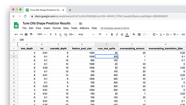
In the remaining code blocks in this section I’ll be discussing the 7 most important hyperparameters you can tune/set when training your own custom dlib shape predictor. These values are:

1. tree_depth

2. nu

3. cascade_depth

4. feature_pool_size

5. num_test_splits

6. oversampling_amount

7. oversampling_translation_jitter

We’ll begin with grabbing the default dlib shape predictor options:

# grab the default options for dlib's shape predictor
print("[INFO] setting shape predictor options...")
options = dlib.shape_predictor_training_options()

From there, we’ll configure the

tree_depth

# define the depth of each regression tree -- there will be a total
# of 2^tree_depth leaves in each tree; small values of tree_depth
# will be *faster* but *less accurate* while larger values will
# generate trees that are *deeper*, *more accurate*, but will run
# *far slower* when making predictions
options.tree_depth = 4

Here we define the

tree_depth

2^tree_depth

Smaller values of

tree_depth

tree_depth

Typical values for

tree_depth

The next parameter we’re going to explore is

nu

# regularization parameter in the range [0, 1] that is used to help
# our model generalize -- values closer to 1 will make our model fit
# the training data better, but could cause overfitting; values closer
# to 0 will help our model generalize but will require us to have
# training data in the order of 1000s of data points
options.nu = 0.1

The

nu

Values closer to

1

0

nu

0

Typically, for small values of

nu

Our next parameter is the

cascade_depth

# the number of cascades used to train the shape predictor -- this
# parameter has a *dramtic* impact on both the *accuracy* and *output
# size* of your model; the more cascades you have, the more accurate
# your model can potentially be, but also the *larger* the output size
options.cascade_depth = 15

A series of cascades are used to refine and tune the initial predictions from the ERTs — the

cascade_depth

The more cascades you allow for, the larger your model will become (but potentially more accurate). The fewer cascades you allow, the smaller your model will be (but could be less accurate).

The following figure from Kazemi and Sullivan’s paper demonstrates the impact that the

cascade_depth

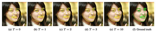
Figure 7: The cascade_depth parameter has a significant impact on the accuracy of your custom dlib shape/landmark predictor model.

Clearly you can see that the deeper the cascade, the better the facial landmark alignment.

Typically you’ll want to explore

cascade_depth

Let’s now move on to the

feature_pool_size

# number of pixels used to generate features for the random trees at
# each cascade -- larger pixel values will make your shape predictor
# more accurate, but slower; use large values if speed is not a
# problem, otherwise smaller values for resource constrained/embedded
# devices
options.feature_pool_size = 400

The

feature_pool_size

The more pixels you include, the slower your model will run (but could potentially be more accurate). The fewer pixels you take into account, the faster your model will run (but could also be less accurate).

My recommendation here is that you should use large values for

feature_pools_size

The next parameter we’re going to set is the

num_test_splits

# selects best features at each cascade when training -- the larger
# this value is, the *longer* it will take to train but (potentially)
# the more *accurate* your model will be
options.num_test_splits = 50

The

num_test_splits

The more

num_test_splits

Let’s check out the

oversampling_amount

# controls amount of "jitter" (i.e., data augmentation) when training
# the shape predictor -- applies the supplied number of random
# deformations, thereby performing regularization and increasing the
# ability of our model to generalize
options.oversampling_amount = 5

The

oversampling_amount

Here we are telling dlib to apply a total of

5

You can think of the

oversampling_amount

Typical

oversampling_amount

0

50

Be careful with this parameter! Larger

oversampling_amount

Next comes the

oversampling_translation_jitter

# amount of translation jitter to apply -- the dlib docs recommend
# values in the range [0, 0.5]
options.oversampling_translation_jitter = 0.1

The

oversampling_translation_jitter

Typical values for translation jitter lie in the range [0, 0.5].

The

be_verbose

# tell the dlib shape predictor to be verbose and print out status
# messages our model trains
options.be_verbose = True

Finally, we have the

num_threads

# number of threads/CPU cores to be used when training -- we default
# this value to the number of available cores on the system, but you
# can supply an integer value here if you would like
options.num_threads = multiprocessing.cpu_count()

This parameter is extremely important as it can dramatically speed up the time it takes to train your model!

The more CPU threads/cores you can supply to dlib, the faster your model will train. We’ll default this value to the total number of CPUs on our system; however, you can set this value as any integer (provided it’s less-than-or-equal-to the number of CPUs on your system).

Now that our

options

train_shape_predictor

# log our training options to the terminal
print("[INFO] shape predictor options:")
print(options)

# train the shape predictor
print("[INFO] training shape predictor...")
dlib.train_shape_predictor(args["training"], args["model"], options)

The dlib library accepts (1) the path to our training XML file, (2) the path to our output shape predictor model, and (3) our set of options.

Once trained the shape predictor will be serialized to disk so we can later use it.

While this script may have appeared especially easy, be sure to spend time configuring your options/hyperparameters for optimal performance.

Training the custom dlib shape predictor

We are now ready to train our custom dlib shape predictor!

Make sure you have (1) downloaded the iBUG-300W dataset and (2) used the “Downloads” section of this tutorial to download the source code to this post.

Once you have done so, you are ready to train the shape predictor:

$ python train_shape_predictor.py \
	--training ibug_300W_large_face_landmark_dataset/labels_ibug_300W_train_eyes.xml \
	--model eye_predictor.dat
[INFO] setting shape predictor options...
[INFO] shape predictor options:
shape_predictor_training_options(be_verbose=1, cascade_depth=15, tree_depth=4, num_trees_per_cascade_level=500, nu=0.1, oversampling_amount=5, oversampling_translation_jitter=0.1, feature_pool_size=400, lambda_param=0.1, num_test_splits=50, feature_pool_region_padding=0, random_seed=, num_threads=20, landmark_relative_padding_mode=1)
[INFO] training shape predictor...
Training with cascade depth: 15
Training with tree depth: 4
Training with 500 trees per cascade level.
Training with nu: 0.1
Training with random seed:
Training with oversampling amount: 5
Training with oversampling translation jitter: 0.1
Training with landmark_relative_padding_mode: 1
Training with feature pool size: 400
Training with feature pool region padding: 0
Training with 20 threads.
Training with lambda_param: 0.1
Training with 50 split tests.
Fitting trees...
Training complete
Training complete, saved predictor to file eye_predictor.dat

The entire training process took 9m11s on my 3 GHz Intel Xeon W processor.

To verify that your shape predictor has been serialized to disk, ensure that

eye_predictor.dat

$ ls -lh *.dat
-rw-r--r--@ 1 adrian  staff    18M Dec  4 17:15 eye_predictor.dat

As you can see, the output model is only 18MB — that’s quite the reduction in file size compared to dlib’s standard/default facial landmark predictor which is 99.7MB!

Implementing our shape predictor evaluation script

Now that we’ve trained our dlib shape predictor, we need to evaluate its performance on both our training and testing sets to verify that it’s not overfitting and that our results will (ideally) generalize to our own images outside the training set.

Open up the

evaluate_shape_predictor.py

# import the necessary packages
import argparse
import dlib

# construct the argument parser and parse the arguments
ap = argparse.ArgumentParser()
ap.add_argument("-p", "--predictor", required=True,
	help="path to trained dlib shape predictor model")
ap.add_argument("-x", "--xml", required=True,
	help="path to input training/testing XML file")
args = vars(ap.parse_args())

# compute the error over the supplied data split and display it to
# our screen
print("[INFO] evaluating shape predictor...")
error = dlib.test_shape_predictor(args["xml"], args["predictor"])
print("[INFO] error: {}".format(error))

Lines 2 and 3 indicate that we need both

argparse

dlib

Our command line arguments include:

• --predictor

   : The path to our serialized shape predictor model that we generated via the previous two “Training” sections.

• --xml

   : The path to the input training/testing XML file (i.e. our eyes-only parsed XML files).

When both of these arguments are provided via the command line, dlib will handle evaluation (Line 16). Dlib handles computing the mean average error (MAE) between the predicted landmark coordinates and the ground-truth landmark coordinates.

The smaller the MAE, the better the predictions.

Shape prediction accuracy results

If you haven’t yet, use the “Downloads” section of this tutorial to download the source code and pre-trained shape predictor.

From there, execute the following command to evaluate our eye landmark predictor on the training set:

$ python evaluate_shape_predictor.py --predictor eye_predictor.dat \
	--xml ibug_300W_large_face_landmark_dataset/labels_ibug_300W_train_eyes.xml
[INFO] evaluating shape predictor...
[INFO] error: 3.631152776257545

Here we are obtaining an MAE of ~3.63.

Let’s now run the same command on our testing set:

$ python evaluate_shape_predictor.py --predictor eye_predictor.dat \
	--xml ibug_300W_large_face_landmark_dataset/labels_ibug_300W_test_eyes.xml
[INFO] evaluating shape predictor...
[INFO] error: 7.568211111799696

As you can see the MAE is twice as large on our testing set versus our training set.

If you have any prior experience working with machine learning or deep learning algorithms you know that in most situations, your training loss will be lower than your testing loss. That doesn’t mean that your model is performing badly — instead, it simply means that your model is doing a better job modeling the training data versus the testing data.

Shape predictors are especially interesting to evaluate as it’s not just the MAE that needs to be examined!

You also need to visually validate the results and verify the shape predictor is working as expected — we’ll cover that topic in the next section.

Implementing the shape predictor inference script

Now that we have our shape predictor trained, we need to visually validate that the results look good by applying it to our own example images/video.

In this section we will:

1. Load our trained dlib shape predictor from disk.
2. Access our video stream.
3. Apply the shape predictor to each individual frame.
4. Verify that the results look good.

Let’s get started.

Open up

predict_eyes.py

# import the necessary packages
from imutils.video import VideoStream
from imutils import face_utils
import argparse
import imutils
import time
import dlib
import cv2

# construct the argument parser and parse the arguments
ap = argparse.ArgumentParser()
ap.add_argument("-p", "--shape-predictor", required=True,
	help="path to facial landmark predictor")
args = vars(ap.parse_args())

Lines 2-8 import necessary packages. In particular we will use

imutils

cv2

VideoStream

face_utils

The only command line argument required for this script is the path to our trained facial landmark predictor,

--shape-predictor

Let’s perform three initializations:

# initialize dlib's face detector (HOG-based) and then load our
# trained shape predictor
print("[INFO] loading facial landmark predictor...")
detector = dlib.get_frontal_face_detector()
predictor = dlib.shape_predictor(args["shape_predictor"])

# initialize the video stream and allow the cammera sensor to warmup
print("[INFO] camera sensor warming up...")
vs = VideoStream(src=0).start()
time.sleep(2.0)

Our initializations include:

• Loading the face

  detector

    (Line 19). The detector allows us to find a face in an image/video prior to localizing landmarks on the face. We’ll be using dlib’s HOG + Linear SVM face detector. Alternatively, you could use Haar cascades (great for resource-constrained, embedded devices) or a more accurate deep learning face detector.
• Loading the facial landmark

  predictor

    (Line 20).
• Initializing our webcam stream (Line 24).

Now we’re ready to loop over frames from our camera:

# loop over the frames from the video stream
while True:
	# grab the frame from the video stream, resize it to have a
	# maximum width of 400 pixels, and convert it to grayscale
	frame = vs.read()
	frame = imutils.resize(frame, width=400)
	gray = cv2.cvtColor(frame, cv2.COLOR_BGR2GRAY)

	# detect faces in the grayscale frame
	rects = detector(gray, 0)

Lines 31-33 grab a frame, resize it, and convert to grayscale.

Line 36 applies face detection using dlib’s HOG + Linear SVM algorithm.

Let’s process the faces detected in the frame by predicting and drawing facial landmarks:

# loop over the face detections
	for rect in rects:
		# convert the dlib rectangle into an OpenCV bounding box and
		# draw a bounding box surrounding the face
		(x, y, w, h) = face_utils.rect_to_bb(rect)
		cv2.rectangle(frame, (x, y), (x + w, y + h), (0, 255, 0), 2)

		# use our custom dlib shape predictor to predict the location
		# of our landmark coordinates, then convert the prediction to
		# an easily parsable NumPy array
		shape = predictor(gray, rect)
		shape = face_utils.shape_to_np(shape)

		# loop over the (x, y)-coordinates from our dlib shape
		# predictor model draw them on the image
		for (sX, sY) in shape:
			cv2.circle(frame, (sX, sY), 1, (0, 0, 255), -1)

Line 39 begins a loop over the detected faces. Inside the loop, we:

• Take dlib’s

  rectangle

  object and convert it to OpenCV’s standard

  (x, y, w, h)

  bounding box ordering (Line 42).
• Draw the bounding box surrounding the face (Line 43).
• Use our custom dlib shape

  predictor

    to predict the location of our landmarks (i.e., eyes) via Line 48.
• Convert the returned coordinates to a NumPy array (Line 49).
• Loop over the predicted landmark coordinates and draw them individually as small dots on the output frame (Line 53 and 54).

If you need a refresher on drawing rectangles and solid circles, refer to my OpenCV Tutorial.

To wrap up we’ll display the result!

# show the frame
	cv2.imshow("Frame", frame)
	key = cv2.waitKey(1) & 0xFF

	# if the `q` key was pressed, break from the loop
	if key == ord("q"):
		break

# do a bit of cleanup
cv2.destroyAllWindows()
vs.stop()

Lines 57 displays the frame to the screen.

If the

q

Making predictions with our dlib shape predictor

Are you ready to see our custom shape predictor in action?

If so, make sure you use the “Downloads” section of this tutorial to download the source code and pre-trained dlib shape predictor.

From there you can execute the following command:

$ python predict_eyes.py --shape-predictor eye_predictor.dat
[INFO] loading facial landmark predictor...
[INFO] camera sensor warming up...

As you can see, our shape predictor is both:

• Correctly localizing my eyes in the input video stream
• Running in real-time

Again, I’d like to call your attention back to the “Balancing shape predictor model speed and accuracy” section of this tutorial — our model is not predicting all of the possible 68 landmark locations on the face!

Instead, we have trained a custom dlib shape predictor that only localizes the eye regions. (i.e., our model is not trained on the other facial structures in the iBUG-300W dataset including i.e., eyebrows, nose, mouth, and jawline).

Our custom eye predictor can be used in situations where we don’t need the additional facial structures and only require the eyes, such as building an a drowsiness detector, building a virtual makeover application for eyeliner/mascara, or creating computer-assisted software to help disabled users utilize their computers.

In next week’s tutorial, I’ll show you how to tune the hyperparameters to dlib’s shape predictor to obtain optimal performance.

How do I create my own dataset for shape predictor training?

To create your own shape predictor dataset you’ll need to use dlib’s imglab tool. Covering how to create and annotate your own dataset for shape predictor training is outside the scope of this blog post. I’ll be covering it in a future tutorial here on PyImageSearch.

What’s next?

Are you interested in learning more about Computer Vision, OpenCV, and the Dlib library?

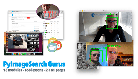
If so, you’ll want to take a look at the PyImageSearch Gurus course.

Inside PyImageSearch Gurus, you’ll find:

• An actionable, real-world course on Computer Vision, Deep Learning, and OpenCV. Each lesson in PyImageSearch Gurus is taught in the same hands-on, easy-to-understand PyImageSearch style that you know and love.
• The most comprehensive computer vision education online today. The PyImageSearch Gurus course covers 13 modules broken out into 168 lessons, with other 2,161 pages of content. You won’t find a more detailed computer vision course anywhere else online, I guarantee it.
• A community of like-minded developers, researchers, and students just like you, who are eager to learn computer vision and level-up their skills.
• Access to private course forums which I personally participate in nearly every day. These forums are a great way to get expert advice, both from me as well as the more advanced students.

To learn more about the course, and grab the course syllabus PDF, just use this link:

Summary

In this tutorial, you learned how to train your own custom dlib shape/landmark predictor.

To train our shape predictor we utilized the iBUG-300W dataset, only instead of training our model to recognize all facial structures (i.e., eyes, eyebrows, nose, mouth, and jawline), we instead trained the model to localize just the eyes.

The end result is a model that is:

• Accurate: Our shape predictor can accurately predict/localize the location of the eyes on a face.
• Small: Our eye landmark predictor is smaller than the pre-trained dlib face landmark predictor (18MB vs. 99.7MB, respectively).
• Fast: Our model is faster than dlib’s pre-trained facial landmark predictor as it predicts fewer locations (the hyperparameters to the model were also chosen to improve speed as well).

In next week’s tutorial, I’ll teach you how to systemically tune the hyperparameters to dlib’s shape predictor training procedure to balance prediction speed, model size, and localization accuracy.

To download the source code to this post (and be notified when future tutorials are published here on PyImageSearch), just enter your email address in the form below!

Downloads:

If you would like to download the code and images used in this post, please enter your email address in the form below. Not only will you get a .zip of the code, I’ll also send you a FREE 17-page Resource Guide on Computer Vision, OpenCV, and Deep Learning. Inside you'll find my hand-picked tutorials, books, courses, and libraries to help you master CV and DL! Sound good? If so, enter your email address and I’ll send you the code immediately!

Email address:

Website

The post Training a custom dlib shape predictor appeared first on PyImageSearch.

In this tutorial, you will learn how to optimally tune dlib’s shape predictor hyperparameters and options to obtain a shape predictor that balances speed, accuracy, and model size.

Today is part two in our two-part series on training custom shape predictors with dlib:

1. Part #1: Training custom dlib shape predictors (last week’s tutorial)
2. Part #2: Tuning dlib shape predictor hyperparameters to balance speed, accuracy, and model size (today’s tutorial)

Many software developers and project managers are familiar with the concept of the “Iron Triangle”. When building software we need to balance:

1. Good, high-quality software
2. Software that can be delivered to the customer fast
3. How expensive the software is (i.e., whether or not it’s cheap)

The caveat is that we can only pick two of the above.

Good, high-quality software that is delivered to the customer quickly is certainly not cheap. Similarly, software that was developed cheaply and delivered fast is likely not good.

When training our own custom dlib shape predictors we have a similar problem — we need to balance:

• Speed: How fast the model can make predictions (i.e., inference speed).
• Accuracy: How precise and accurate our model is in its predictions.
• Model size: The larger the model is, the more space it takes up, and the more computational resources it requires. Smaller models are therefore preferred.

But unlike the Iron Triangle of software development which only has three vertices, dlib’s shape predictor includes 7-10 options that you’ll typically want to tune.

So, how do we go about tuning these shape predictor options and hyperparameters?

I’ll be discussing that topic in the remainder of the post.

Note: If you haven’t read last week’s post on training a dlib shape predictor, make sure you do so now, as the rest of this tutorial builds on it.

To learn how to tune dlib’s shape predictor options to optimally balance speed, accuracy, and model size, just keep reading!

Tuning dlib shape predictor hyperparameters to balance speed, accuracy, and model size

In the first part of this tutorial, we’ll discuss why we need to tune the options to dlib’s shape predictor to obtain an optimal model for our particular project requirements and application.

From there we’ll review discuss the dataset we’ll be using today to train our dlib shape predictor on.

I’ll then show you how you can implement a Python script to automatically explore dlib’s shape predictor options.

We’ll wrap up the tutorial by discussing how we can use the results of this script to set the options to dlib’s shape predictor, train it, and obtain an optimal model.

Let’s get started!

Why do we need to tune our shape predictor hyperparameters?

Figure 1: In this tutorial, we will learn how to tune custom dlib shape predictor hyperparameters to balance speed, accuracy, and model size.

When training our own custom dlib shape predictors we need to balance:

• Model speed
• Model accuracy
• Model size

Typically we can only have 1-2 of these choices.

Before you even open up your code editor or command line, first consider the goal of the project and where you shape predictor will be deployed:

• Will the shape predictor be used on an embedded device? If so, compromise on accuracy a bit and seek a model that is fast and small.
• Are you deploying the model to modern laptop/desktops? You may be able to get away with larger models that are more computationally expensive so don’t worry as much about model size and focus on maximizing accuracy.
• Is the output size of the model a concern? If your model needs to be deployed/updated over a network connection then you should seek a model that is as small as possible but still achieves reasonable accuracy.
• Is the amount of time it takes to train the model a concern? If so, pay attention to any jitter/data augmentation applied during the training process.

Considering these options ahead of time will make it far easier for you to tune the options to dlib’s shape predictor — I’ll also show you my own tuning script that I use to help narrow in on shape predictor options that will work well for my respective use cases.

The iBUG-300W dataset

Figure 2: The iBug 300-W face landmark dataset is used to train a custom dlib shape predictor. We will tune custom dlib shape predictor hyperparameters in an effort to balance speed, accuracy, and model size.

To train and tune our own custom dlib shape predictors, we’ll be using the iBUG 300-W dataset, the same dataset we used in last week’s tutorial.

The iBUG 300-W dataset is used to train facial landmark predictors and localize the individual structures of the face, including:

• Eyebrows
• Eyes
• Nose
• Mouth
• Jawline

However, we’ll be training our shape predictor to localize only the eyes — our model will not be trained on the other facial structures.

For more details on the iBUG 300-W dataset, refer to last week’s blog post.

Configuring your dlib development environment

To follow along with today’s tutorial, you will need a virtual environment with the following packages installed:

• dlib
• OpenCV
• imutils
• scikit-learn

Luckily, each of these packages is pip-installable, but there are a handful of pre-requisites (including Python virtual environments). Be sure to follow these two guides for additional information in configuring your development environment:

• Install dlib (the easy, complete guide)
• pip install opencv

The pip install commands include:

$ workon <env-name>
$ pip install dlib
$ pip install opencv-contrib-python
$ pip install imutils
$ pip install scikit-learn

The

workon

virtualenv

virtualenvwrapper

Downloading the iBUG 300-W dataset

Before we get too far into this tutorial, take a second now to download the iBUG 300-W dataset (~1.7GB):

http://dlib.net/files/data/ibug_300W_large_face_landmark_dataset.tar.gz

You’ll also want to use the “Downloads” section of this blog post to download the source code.

I recommend placing the iBug 300-W dataset into the zip associated with the download of this tutorial like this:

$ unzip tune-dlib-shape-predictor.zip
...
$ cd tune-dlib-shape-predictor
$ mv ~/Downloads/ibug_300W_large_face_landmark_dataset.tar.gz .
$ tar -xvf ibug_300W_large_face_landmark_dataset.tar.gz
...

Alternatively (i.e. rather than clicking the hyperlink above), use

wget

$ unzip tune-dlib-shape-predictor.zip
...
$ cd tune-dlib-shape-predictor
$ wget http://dlib.net/files/data/ibug_300W_large_face_landmark_dataset.tar.gz
$ tar -xvf ibug_300W_large_face_landmark_dataset.tar.gz
...

From there you can follow along with the rest of the tutorial.

Project structure

Assuming you have followed the instructions in the previous section, your project directory is now organized as follows:

$ tree --dirsfirst --filelimit 15
.
├── ibug_300W_large_face_landmark_dataset
│   ├── afw [1011 entries]
│   ├── helen
│   │   ├── testset [990 entries]
│   │   └── trainset [6000 entries]
│   ├── ibug [405 entries]
│   ├── image_metadata_stylesheet.xsl
│   ├── labels_ibug_300W.xml
│   ├── labels_ibug_300W_test.xml
│   ├── labels_ibug_300W_train.xml
│   └── lfpw
│       ├── testset [672 entries]
│       └── trainset [2433 entries]
├── ibug_300W_large_face_landmark_dataset.tar.gz
├── pyimagesearch
│   ├── __init__.py
│   └── config.py
├── example.jpg
├── ibug_300W_large_face_landmark_dataset.tar.gz
├── optimal_eye_predictor.dat
├── parse_xml.py
├── predict_eyes.py
├── train_shape_predictor.py
├── trials.csv
└── tune_predictor_hyperparams.py

2 directories, 15 files

Last week, we reviewed the following Python scripts:

• parse_xml.py

  : Parses the train/test XML dataset files for eyes-only landmark coordinates.

• train_shape_predictor.py

   : Accepts the parsed XML files to train our shape predictor with dlib.

• evaluate_shape_predictor.py

  : Calculates the Mean Average Error (MAE) of our custom shape predictor. Not included in today’s download — similar/additional functionality is provided in today’s tuning script.

• predict_eyes.py

  : Performs shape prediction using our custom dlib shape predictor, trained to only recognize eye landmarks.

Today we will review the following Python files:

• config.py

   : Our configuration paths, constants, and variables are all in one convenient location.

• tune_predictor_hyperparams.py

   : The heart of today’s tutorial lays here. This script determines all 6,075 combinations of dlib shape predictor hyperparameters. From there, we’ll randomly sample 100 combinations and proceed to train and evaluate those 100 models. The hyperparameters and evaluation criteria are output to a CSV file for inspection in a spreadsheet application of your choice.

Preparing the iBUG-300W dataset for training

Figure 3: Our custom dlib shape/landmark predictor recognizes just eyes.

As mentioned in the “The iBUG-300W dataset” section above, we’ll be training our dlib shape predictor on just the eyes (i.e., not the eyebrows, nose, mouth or jawline).

To accomplish that task, we first need to parse out any facial structures we are not interested in from the iBUG 300-W training/testing XML files.

To get started, make sure you’ve:

1. Used the “Downloads” section of this tutorial to download the source code.
2. Used the “Downloading the iBUG-300W dataset” section above to download the iBUG-300W dataset.
3. Reviewed the “Project structure” section.

You’ll notice inside your directory structure for the project that there is a script named

parse_xml.py

We reviewed this file in detail in last week’s tutorial so we’re not going to review it again here today (refer to last week’s post to understand how it works).

Before you continue on with the rest of this tutorial you’ll need to execute the following command to prepare our “eyes only” training and testing XML files:

$ python parse_xml.py \
	--input ibug_300W_large_face_landmark_dataset/labels_ibug_300W_train.xml \
	--output ibug_300W_large_face_landmark_dataset/labels_ibug_300W_train_eyes.xml
[INFO] parsing data split XML file...
$ python parse_xml.py \
	--input ibug_300W_large_face_landmark_dataset/labels_ibug_300W_test.xml \
	--output ibug_300W_large_face_landmark_dataset/labels_ibug_300W_test_eyes.xml
[INFO] parsing data split XML file...

To verify that our new training/testing files have been created, check your iBUG-300W root dataset directory for the

labels_ibug_300W_train_eyes.xml

labels_ibug_300W_test_eyes.xml

$ cd ibug_300W_large_face_landmark_dataset
$ ls -lh *.xml    
-rw-r--r--@ 1 adrian  staff    21M Aug 16  2014 labels_ibug_300W.xml
-rw-r--r--@ 1 adrian  staff   2.8M Aug 16  2014 labels_ibug_300W_test.xml
-rw-r--r--  1 adrian  staff   602K Dec 12 12:54 labels_ibug_300W_test_eyes.xml
-rw-r--r--@ 1 adrian  staff    18M Aug 16  2014 labels_ibug_300W_train.xml
-rw-r--r--  1 adrian  staff   3.9M Dec 12 12:54 labels_ibug_300W_train_eyes.xml
$ cd ..

Notice that our

*_eyes.xml

Once you have performed these steps you can continue on with the rest of the tutorial.

Reviewing our configuration file

Before we get too far in this project, let’s first review our configuration file.

Open up the

config.py

# import the necessary packages
import os

# define the path to the training and testing XML files
TRAIN_PATH = os.path.join("ibug_300W_large_face_landmark_dataset",
	"labels_ibug_300W_train_eyes.xml")
TEST_PATH = os.path.join("ibug_300W_large_face_landmark_dataset",
	"labels_ibug_300W_test_eyes.xml")

Here we have the paths to training and testing XML files (i.e. the ones generated after we have parsed out the eye regions).

Next, we’ll define a handful of constants for tuning dlib shape predictor hyperparameters:

# define the path to the temporary model file
TEMP_MODEL_PATH = "temp.dat"

# define the path to the output CSV file containing the results of
# our experiments
CSV_PATH = "trials.csv"

# define the path to the example image we'll be using to evaluate
# inference speed using the shape predictor
IMAGE_PATH = "example.jpg"

# define the number of threads/cores we'll be using when trianing our
# shape predictor models
PROCS = -1

# define the maximum number of trials we'll be performing when tuning
# our shape predictor hyperparameters
MAX_TRIALS = 100

Our dlib tuning paths include:

• Our temporary shape predictor file used during option/hyperparameter tuning (Line 11).
• The CSV file used to store the results of our individual trials (Line 15).
• An example image we’ll be using to evaluate a given model’s inference speed (Line 19).

Next, we’ll define a multiprocessing variable — the number of parallel threads/cores will be using when training our shape predictor (Line 23). A value of

-1

We’ll be working through combinations of hyperparameters to find the best performing model. Line 27 defines the maximum number of trials we’ll be performing when exploring the shape predictor hyperparameter space:

• Smaller values will result in the

  tune_predictor_hyperparams.py

  script completing faster, but will also explore fewer options.
• Larger values will require significantly more time for the

  tune_predictor_hyperparams.py

  script to complete and will explore more options, providing you with more results that you can then use to make better, more informed decisions on how to select your final shape predictor hyperparameters.

If we were to find the best model out of 6,000+, it would take multiple weeks/months time to train and evaluate the shape predictor models even on a powerful computer; therefore, you should seek a balance with the

MAX_TRIALS

Implementing our dlib shape predictor tuning script

If you followed last week’s post on training a custom dlib shape predictor, you’ll note that we hardcoded all of the options to our shape predictor.

Hardcoding our hyperparameter values is a bit of a problem as it requires that we manually:

1. Step #1: Update any training options.
2. Step #2: Execute the script used to train the shape predictor.
3. Step #3: Evaluate the newly trained shape predictor on our shape model.
4. Step #4: Go back to Step #1 and repeat as necessary.

The problem here is that these steps are a manual process, requiring us to intervene at each and every step.

Instead, it would be better if we could create a Python script that automatically handles the tuning process for us.

We could define the options and corresponding values we want to explore. Our script would determine all possible combinations of these parameters. It would then train a shape predictor on these options, evaluate it, and then proceed to the next set of options. Once the script completes running we can examine the results, select the best parameters to achieve our balance of model speed, size, and accuracy, and then train the final model.

To learn how we can create such a script, open up the

tune_predictor_hyperparams.py

# import the necessary packages
from pyimagesearch import config
from sklearn.model_selection import ParameterGrid
import multiprocessing
import numpy as np
import random
import time
import dlib
import cv2
import os

Lines 2-10 import our packages including:

• config

   : Our configuration.

• ParameterGrid

  : Generates an iterable list of parameter combinations. Refer to scikit-learn’s Parameter Grid documentation.

• multiprocessing

   : Python’s built-in module for multiprocessing.

• dlib

   : Davis King’s image processing toolkit which includes a shape predictor implementation.

• cv2

  : OpenCV is used today for image I/O and preprocessing.

Let’s now define our function to evaluate our model accuracy:

def evaluate_model_acc(xmlPath, predPath):
	# compute and return the error (lower is better) of the shape
	# predictor over our testing path
	return dlib.test_shape_predictor(xmlPath, predPath)

Lines 12-15 define a helper utility to evaluate our Mean Average Error (MAE), or more simply, the model accuracy.

Just like we have a function that evaluates the accuracy of a model, we also need a method to evaluate the model inference speed:

def evaluate_model_speed(predictor, imagePath, tests=10):
	# initialize the list of timings
	timings = []

	# loop over the number of speed tests to perform
	for i in range(0, tests):
		# load the input image and convert it to grayscale
		image = cv2.imread(config.IMAGE_PATH)
		gray = cv2.cvtColor(image, cv2.COLOR_BGR2GRAY)

		# detect faces in the grayscale frame
		detector = dlib.get_frontal_face_detector()
		rects = detector(gray, 1)

		# ensure at least one face was detected
		if len(rects) > 0:
			# time how long it takes to perform shape prediction
			# using the current shape prediction model
			start = time.time()
			shape = predictor(gray, rects[0])
			end = time.time()

		# update our timings list
		timings.append(end - start)

	# compute and return the average over the timings
	return np.average(timings)

Our

evaluate_model_speed

• predictor

   : The path to the dlib shape/landmark detector.

• imagePath

   : Path to an input image.

• tests

   : The number of tests to perform and average.

Line 19 initializes a list of

timings

timings

• Load an

  image

    and convert it to grayscale (Lines 24 and 25).
• Perform face detection using dlib’s HOG + Linear SVM face

  detector

    (Lines 28 and 29).
• Ensure at least one face was detected (Line 32).
• Calculate the inference time for shape/landmark prediction and add the result to

  timings

    (Lines 35-40).

Finally, we return our

timings

Let’s define a list of columns for our hyperparameter CSV file:

# define the columns of our output CSV file
cols = [
	"tree_depth",
	"nu",
	"cascade_depth",
	"feature_pool_size",
	"num_test_splits",
	"oversampling_amount",
	"oversampling_translation_jitter",
	"inference_speed",
	"training_time",
	"training_error",
	"testing_error",
	"model_size"
]

Remember, this CSV will hold the values of all the hyperparameters that our script tunes. Lines 46-59 define the columns of the CSV file, including the:

• Hyperparameter values for a given trial:

  • tree_depth

    : Controls the tree depth.

  • nu

    : Regularization parameter to help our model generalize.

  • cascade_depth

    : Number of cascades to refine and tune the initial predictions.

  • feature_pool_size

    : Controls the number of pixels used to generate features for the random trees in the cascade.

  • num_test_splits

    : The number of test splits impacts training time and model accuracy.

  • oversampling_amount

    : Controls the amount of “jitter” to apply when training the shape predictor.

  • oversampling_translation_jitter

    : Controls the amount of translation “jitter”/augmentation applied to the dataset.
• Evaluation criteria:

  • inference_speed

    : Inference speed of the trained shape predictor.

  • training_time

    : Amount of time it took to train the shape predictor.

  • training_error

    : Error on the training set.

  • testing_error

    : Error on the testing set.

  • model_size

    : The model filesize.

Note: Keep reading for a brief review of the hyperparameter values including guidelines on how to initialize them.

We then open our output CSV file and write the

cols

# open the CSV file for writing and then write the columns as the
# header of the CSV file
csv = open(config.CSV_PATH, "w")
csv.write("{}\n".format(",".join(cols)))

# determine the number of processes/threads to use
procs = multiprocessing.cpu_count()
procs = config.PROCS if config.PROCS > 0 else procs

Lines 63 and 64 write the

cols

Lines 67 and 68 determine the number of processes/threads to use when training. This number is based on the number of CPUs/cores your machine has. My 3GHz Intel Xeon W has 20 cores, but most laptop CPUs will have 2-8 cores.

The next code block initializes the set hyperparameters/options as well as corresponding values that we’ll be exploring:

# initialize the list of dlib shape predictor hyperparameters that
# we'll be tuning over
hyperparams = {
	"tree_depth": list(range(2, 8, 2)),
	"nu": [0.01, 0.1, 0.25],
	"cascade_depth": list(range(6, 16, 2)),
	"feature_pool_size": [100, 250, 500, 750, 1000],
	"num_test_splits": [20, 100, 300],
	"oversampling_amount": [1, 20, 40],
	"oversampling_translation_jitter": [0.0, 0.1, 0.25]
}

As discussed in last week’s post, there are 7 shape predictor options you’ll want to explore.

We reviewed in them in detail last week, but you can find a short summary of each below:

• tree_depth

  : There will be

  2^tree_depth

  leaves in each tree. Smaller values of

  tree_depth

  will lead to more shallow trees that are faster, but potentially less accurate. Larger values of

  tree_depth

  will create deeper trees that are slower, but potentially more accurate.

• nu

  : Regularization parameter used to help our model generalize. Values closer to

  1

  will make our model fit the training data closer, but could potentially lead to overfitting. Values closer to

  0

  will help our model generalize; however, there is a caveat there — the closer

  nu

  is to

  0

  the more training data you will need.

• cascade_depth

  : Number of cascades used to refine and tune the initial predictions. This parameter will have a dramatic impact on both the accuracy and the output file size of the model. The more cascades you allow, the larger your model will become (and potentially more accurate). The fewer cascades you allow, the smaller your model will be (but could also result in less accuracy).

• feature_pool_size

  : Controls the number of pixels used to generate features for each of the random trees in the cascade. The more pixels you include, the slower your model will run (but could also result in a more accurate shape predictor). The fewer pixels you take into account, the faster your model will run (but could also be less accurate).

• num_test_splits

  : Impacts both training time and model accuracy. The more

  num_test_splits

  you consider, the more likely you’ll have an accurate shape predictor, but be careful! Large values will cause training time to explode and take much longer for the shape predictor training to complete.

• oversampling_amount

  : Controls the amount of “jitter” (i.e., data augmentation) to apply when training the shape predictor. Typical values lie in the range [0, 50]. A value of

  5

  , for instance, would result in a 5x increase in your training data. Be careful here as the larger the

  oversampling_amount

  , the longer it will take your model to train.

• oversampling_translation_jitter

  : Controls the amount of translation jitter/augmentation applied to the dataset.

Now that we have the set of

hyperparams

ParameterGrid

# construct the set of hyperparameter combinations and randomly
# sample them as trying to test *all* of them would be
# computationally prohibitive
combos = list(ParameterGrid(hyperparams))
random.shuffle(combos)
sampledCombos = combos[:config.MAX_TRIALS]
print("[INFO] sampling {} of {} possible combinations".format(
	len(sampledCombos), len(combos)))

Given our set of

hyperparams

On a single machine that would take weeks to explore so we’ll instead randomly sample the parameters to get a reasonable coverage of the possible values.

Lines 85 and 86 constructs the set of all possible option/value combinations and randomly shuffles them. We then sample

MAX_TRIALS

Let’s go ahead and loop over our

sampledCombos

# loop over our hyperparameter combinations
for (i, p) in enumerate(sampledCombos):
	# log experiment number
	print("[INFO] starting trial {}/{}...".format(i + 1,
		len(sampledCombos)))
	
	# grab the default options for dlib's shape predictor and then
	# set the values based on our current hyperparameter values
	options = dlib.shape_predictor_training_options()
	options.tree_depth = p["tree_depth"]
	options.nu = p["nu"]
	options.cascade_depth = p["cascade_depth"]
	options.feature_pool_size = p["feature_pool_size"]
	options.num_test_splits = p["num_test_splits"]
	options.oversampling_amount = p["oversampling_amount"]
	otj = p["oversampling_translation_jitter"]
	options.oversampling_translation_jitter = otj

	# tell dlib to be verbose when training and utilize our supplied
	# number of threads when training
	options.be_verbose = True
	options.num_threads = procs

Line 99 grabs the default

options

Lines 100-107 set each of the dlib shape predictor hyperparameter

options

Lines 111 and 112 tell dlib to be verbose when training and use the configured number of threads (refer to Lines 67 and 68 regarding the number of threads/processes).

From here we will train and evaluate our shape predictor with dlib:

# train the model using the current set of hyperparameters
	start = time.time()
	dlib.train_shape_predictor(config.TRAIN_PATH,
		config.TEMP_MODEL_PATH, options)
	trainingTime = time.time() - start

	# evaluate the model on both the training and testing split
	trainingError = evaluate_model_acc(config.TRAIN_PATH,
		config.TEMP_MODEL_PATH)
	testingError = evaluate_model_acc(config.TEST_PATH,
		config.TEMP_MODEL_PATH)

	# compute an approximate inference speed using the trained shape
	# predictor
	predictor = dlib.shape_predictor(config.TEMP_MODEL_PATH)
	inferenceSpeed = evaluate_model_speed(predictor,
		config.IMAGE_PATH)

	# determine the model size
	modelSize = os.path.getsize(config.TEMP_MODEL_PATH)

Lines 115-118 train our custom dlib shape predictor, including calculating the elapsed training time.

We then use the newly trained shape predictor to compute the error on our training and testing splits, respectively (Lines 121-124).

To estimate the

inferenceSpeed

Line 133 grabs the filesize of the model.

Next, we’ll output the hyperparameter options and evaluation metrics to the CSV file:

# build the row of data that will be written to our CSV file
	row = [
		p["tree_depth"],
		p["nu"],
		p["cascade_depth"],
		p["feature_pool_size"],
		p["num_test_splits"],
		p["oversampling_amount"],
		p["oversampling_translation_jitter"],
		inferenceSpeed,
		trainingTime,
		trainingError,
		testingError,
		modelSize,
	]
	row = [str(x) for x in row]

	# write the output row to our CSV file
	csv.write("{}\n".format(",".join(row)))
	csv.flush()

	# delete the temporary shape predictor model
	if os.path.exists(config.TEMP_MODEL_PATH):
		os.remove(config.TEMP_MODEL_PATH)

# close the output CSV file
print("[INFO] cleaning up...")
csv.close()

Lines 136-150 generates a string-based list of the training hyperparameters and evaluation results.

We then write the row to disk, delete the temporary model file, and cleanup (Lines 153-162).

Again, this loop will run for a maximum of

100

Exploring the shape predictor hyperparameter space

Now that we’ve implemented our Python script to explore dlib’s shape predictor hyperparameter space, let’s put it to work.

Make sure you have:

1. Used the “Downloads” section of this tutorial to download the source code.
2. Downloaded the iBUG-300W dataset using the “Downloading the iBUG-300W dataset” section above.
3. Executed the

   parse_xml.py

   for both the training and testing XML files in the “Preparing the iBUG-300W dataset for training” section.

Provided you have accomplished each of these steps, you can now execute the

tune_predictor_hyperparams.py

$ python tune_predictor_hyperparams.py
[INFO] sampling 100 of 6075 possible combinations
[INFO] starting trial 1/100...
...
[INFO] starting trial 100/100...
Training with cascade depth: 12
Training with tree depth: 4
Training with 500 trees per cascade level.
Training with nu: 0.25
Training with random seed:
Training with oversampling amount: 20
Training with oversampling translation jitter: 0.1
Training with landmark_relative_padding_mode: 1
Training with feature pool size: 1000
Training with feature pool region padding: 0
Training with 20 threads.
Training with lambda_param: 0.1
Training with 100 split tests.
Fitting trees...
Training complete
Training complete, saved predictor to file temp.dat
[INFO] cleaning up...

real    3052m50.195s
user    30926m32.819s
sys     338m44.848s

On my iMac Pro with a 3GHz Intel Xeon W processor, the entire training time took ~3,052 minutes which equates to ~2.11 days. Be sure to run the script overnight and plan to check the status in 2-5 days depending on your computational horsepower.

After the script completes, you should now have a file named

trials.csv

$ ls *.csv
trials.csv

Our

trials.csv

In the next section, we’ll examine this file and use it to select optimal shape predictor options that balance speed, accuracy, and model size.

Determining the optimal shape predictor parameters to balance speed, accuracy, and model size

At this point, we have our output

trials.csv

Our goal here is to analyze this CSV file and determine the most appropriate values for our particular task.

To get started, open up this CSV file in your favorite spreadsheet application (ex., Microsoft Excel, macOS Numbers, Google Sheets, etc.):

Figure 4: Hyperparameter tuning a dlib shape predictor produced the following data to analyze in a spreadsheet. We will analyze hyperparameters and evaluation criteria to balance speed, accuracy, and shape predictor model size.

Let’s now suppose that my goal is to train and deploy a shape predictor to an embedded device.

For embedded devices, our model should:

• Be as small as possible
• A small model will also be fast when making predictions, a requirement when working with resource-constrained devices
• Have reasonable accuracy, but understanding that we need to sacrifice accuracy a bit to have a small, fast model.

To identify the optimal hyperparameters for dlib’s shape predictor, I would first sort my spreadsheet by model size:

Figure 5: Sort your dlib shape predictors by model size when you are analyzing the results of tuning your model to balance speed, accuracy, and model size.

I would then examine the

inference_speed

training_error

testing_error

Doing so, I find the following model, bolded and selected in the spreadsheet:

Figure 6: After sorting your dlib shape predictor turning by model_size, examine the inference_speed, training_error, and testing_error columns, looking for a model that is fast but also has reasonable accuracy.

This model is:

• Only 3.85MB in size
• In the top-25 in terms of testing error
• Extremely fast, capable of performing 1,875 predictions in a single second

Below I’ve included the shape predictor hyperparameters for this model:

• tree_depth

  : 2

• nu

  : 0.25

• cascade_depth

  : 12

• feature_pool_size

  : 500

• num_test_splits

  : 100

• oversampling_amount

  : 20

• oversampling_translation_jitter

  : 0

Updating our shape predictor training script

We’re almost done!

The last update we need to make is to our

train_shape_predictor.py

Open up that file and insert the following code:

# import the necessary packages
import multiprocessing
import argparse
import dlib

# construct the argument parser and parse the arguments
ap = argparse.ArgumentParser()
ap.add_argument("-t", "--training", required=True,
	help="path to input training XML file")
ap.add_argument("-m", "--model", required=True,
	help="path serialized dlib shape predictor model")
args = vars(ap.parse_args())

# grab the default options for dlib's shape predictor
print("[INFO] setting shape predictor options...")
options = dlib.shape_predictor_training_options()

# update our hyperparameters
options.tree_depth = 2
options.nu = 0.25
options.cascade_depth = 12
options.feature_pool_size = 500
options.num_test_splits = 20
options.oversampling_amount = 20
options.oversampling_translation_jitter = 0

# tell the dlib shape predictor to be verbose and print out status
# messages our model trains
options.be_verbose = True

# number of threads/CPU cores to be used when training -- we default
# this value to the number of available cores on the system, but you
# can supply an integer value here if you would like
options.num_threads = multiprocessing.cpu_count()

# log our training options to the terminal
print("[INFO] shape predictor options:")
print(options)

# train the shape predictor
print("[INFO] training shape predictor...")
dlib.train_shape_predictor(args["training"], args["model"], options)

Notice how on Lines 19-25 we have updated our shape predictor options using the optimal values we found in the previous section.

The rest of our script takes care of training the shape predictor using these values.

For a detailed review of the the

train_shape_predictor.py

Training the dlib shape predictor on our optimal option values

Now that we’ve identified our optimal shape predictor options, as well as updated our

train_shape_predictor.py

Open up a terminal and execute the following command:

$ time python train_shape_predictor.py \
	--training ibug_300W_large_face_landmark_dataset/labels_ibug_300W_train_eyes.xml \
	--model optimal_eye_predictor.dat
[INFO] setting shape predictor options...
[INFO] shape predictor options:
shape_predictor_training_options(be_verbose=1, cascade_depth=12, tree_depth=2, num_trees_per_cascade_level=500, nu=0.25, oversampling_amount=20, oversampling_translation_jitter=0, feature_pool_size=500, lambda_param=0.1, num_test_splits=20, feature_pool_region_padding=0, random_seed=, num_threads=20, landmark_relative_padding_mode=1)
[INFO] training shape predictor...
Training with cascade depth: 12
Training with tree depth: 2
Training with 500 trees per cascade level.
Training with nu: 0.25
Training with random seed: 
Training with oversampling amount: 20
Training with oversampling translation jitter: 0
Training with landmark_relative_padding_mode: 1
Training with feature pool size: 500
Training with feature pool region padding: 0
Training with 20 threads.
Training with lambda_param: 0.1
Training with 20 split tests.
Fitting trees...
Training complete                             
Training complete, saved predictor to file optimal_eye_predictor.dat

real	10m49.273s
user	83m6.673s
sys		0m47.224s

Once trained, we can use the

predict_eyes.py

As you can see, we have trained a dlib shape predictor that:

• Accurately localizes eyes
• Is fast in terms of inference/prediction speed
• Is small in terms of model size

You can perform the same analysis when training your own custom dlib shape predictors as well.

How can we speed up our shape predictor tuning script?

Figure 7: Tuning dlib shape predictor hyperparameters allows us to balance speed, accuracy, and model size.

The obvious bottleneck here is the

tune_predictor_hyperparams.py

Exploring all of the possible hyperparameters would therefore take months!

And keep in mind that we’re training an eyes-only landmark predictor. Had we been training models for all 68 typical landmarks, training would take even longer.

In most cases we simply won’t have that much time (or patience).

So, what can we do about it?

To start, I would suggest reducing your hyperparameter space.

For example, let’s assume you are training a dlib shape predictor model to be deployed to an embedded device such as the Raspberry Pi, Google Coral, or NVIDIA Jetson Nano. In those cases you’ll want a model that is fast and small — you therefore know you’ll need to comprise a bit of accuracy to obtain a fast and small model.

In that situation, you’ll want to avoid exploring areas of the hyperparameter space that will result in models that are larger and slower to make predictions. Consider limiting your

tree_depth

cascade_depth

feature_pool_size

Do not confuse deployment with training. You should tune/train your shape predictor on a capable, full-size machine (i.e. not an embedded device). From there, assuming your model is reasonably small for an embedded device, you should then deploy the model to the target device.

Secondly, I would suggest leveraging distributed computing.

Tuning hyperparameters to a model is a great example of a problem that scales linearly and can be solved by throwing more hardware at it.

For example, you could use Amazon, Microsoft, Google’s etc. cloud to spin up multiple machines. Each machine can then be responsible for exploring non-overlapping subsets of the hyperparameters. Given N total machines, you can reduce the amount of time it takes to tune your shape predictor options by a factor of N.

Of course, we might not have the budget to leverage the cloud, in which case, you should see my first suggestion above.

Expand your computer vision knowledge in the PyImageSearch Gurus Course and Community

Are you overwhelmed with the many Python libraries for computer vision, deep learning, machine learning, and data science?

We’ve all been there when we first started. What you need to do is put one foot in front of the other and just get started In order to help you expand your Computer Vision knowledge and skillset, I have put together the PyImageSearch Gurus course.

Inside the course you’ll learn:

• Machine learning and image classification
• Automatic License/Number Plate Recognition (ANPR)
• Face recognition
• How to train HOG + Linear SVM object detectors with dlib
• Content-based Image Retrieval (i.e., image search engines)
• Processing image datasets with Hadoop and MapReduce
• Hand gesture recognition
• Deep learning fundamentals
• …and much more!

PyImageSearch Gurus is the most comprehensive computer vision education online today, covering 13 modules broken out into 168 lessons, with other 2,161 pages of content. You won’t find a more detailed computer vision course anywhere else online, I guarantee it.

The learning does not stop with the course. PyImageSearch Gurus also includes private community forums. I participate in the Gurus forum virtually nearly every day, so it’s a great way to gain expert advice, both from me and from the other advanced students, on a daily basis.

To learn more about the PyImageSearch Gurus course + community (and grab 10 FREE sample lessons), just click the button below:

Summary

In this tutorial you learned how to automatically tune the options and hyperparameters to dlib’s shape predictor, allowing you to properly balance:

1. Model inference/prediction speed
2. Model accuracy
3. Model size

Tuning hyperparameters is very computationally expensive, so it’s recommended that you either:

• Budget enough time (2-4 days) on your personal laptop or desktop to run the hyperparameter tuning script.
• Utilize distributed systems and potentially the cloud to spin up multiple systems, each of which crunches on non-overlapping subsets of the hyperparameters.

After the tuning script runs you can open up the resulting CSV/Excel file, sort it by which columns you are most interested in (i.e., speed, accuracy, size), and determine your optimal hyperparameters.

Given the parameters, you found from your sorting you can then update the shape predictor training script and then train your model.

I hope you enjoyed today’s tutorial!

To download the source code to this post (and be notified when future tutorials are published here on PyImageSearch), just enter your email address in the form below!

Downloads:

If you would like to download the code and images used in this post, please enter your email address in the form below. Not only will you get a .zip of the code, I’ll also send you a FREE 17-page Resource Guide on Computer Vision, OpenCV, and Deep Learning. Inside you'll find my hand-picked tutorials, books, courses, and libraries to help you master CV and DL! Sound good? If so, enter your email address and I’ll send you the code immediately!

Email address:

Website

The post Tuning dlib shape predictor hyperparameters to balance speed, accuracy, and model size appeared first on PyImageSearch.

In this tutorial, you will learn two ways to implement label smoothing using Keras, TensorFlow, and Deep Learning.

When training your own custom deep neural networks there are two critical questions that you should constantly be asking yourself:

1. Am I overfitting to my training data?
2. Will my model generalize to data outside my training and testing splits?

Regularization methods are used to help combat overfitting and help our model generalize. Examples of regularization methods include dropout, L2 weight decay, data augmentation, etc.

However, there is another regularization technique we haven’t discussed yet — label smoothing.

Label smoothing:

• Turns “hard” class label assignments to “soft” label assignments.
• Operates directly on the labels themselves.
• Is dead simple to implement.
• Can lead to a model that generalizes better.

In the remainder of this tutorial, I’ll show you how to implement label smoothing and utilize it when training your own custom neural networks.

To learn more about label smoothing with Keras and TensorFlow, just keep reading!

Label smoothing with Keras, TensorFlow, and Deep Learning

In the first part of this tutorial I’ll address three questions:

1. What is label smoothing?
2. Why would we want to apply label smoothing?
3. How does label smoothing improve our output model?

From there I’ll show you two methods to implement label smoothing using Keras and TensorFlow:

1. Label smoothing by explicitly updating your labels list
2. Label smoothing using your loss function

We’ll then train our own custom models using both methods and examine the results.

What is label smoothing and why would we want to use it?

When performing image classification tasks we typically think of labels as hard, binary assignments.

For example, let’s consider the following image from the MNIST dataset:

Figure 1: Label smoothing with Keras, TensorFlow, and Deep Learning is a regularization technique with a goal of enabling your model to generalize to new data better.

This digit is clearly a “7”, and if we were to write out the one-hot encoded label vector for this data point it would look like the following:

[0.0, 0.0, 0.0, 0.0, 0.0, 0.0, 0.0, 1.0, 0.0, 0.0]

Notice how we’re performing hard label assignment here: all entries in the vector are

0

1

Hard label assignment is natural to us and maps to how our brains want to efficiently categorize and store information in neatly labeled and packaged boxes.

For example, we would look at Figure 1 and say something like:

“I’m sure that’s a 7. I’m going to label it a 7 and put it in the ‘7’ box.”

It would feel awkward and unintuitive to say the following:

“Well, I’m sure that’s a 7. But even though I’m 100% certain that it’s a 7, I’m going to put 90% of that 7 in the ‘7’ box and then divide the remaining 10% into all boxes just so my brain doesn’t overfit to what a ‘7’ looks like.”

If we were to apply soft label assignment to our one-hot encoded vector above it would now look like this:

[0.01 0.01 0.01 0.01 0.01 0.01 0.01 0.91 0.01 0.01]

Notice how summing the list of values equals

1

This type of label assignment is called soft label assignment.

Unlike hard label assignments where class labels are binary (i.e., positive for one class and a negative example for all other classes), soft label assignment allows:

• The positive class to have the largest probability
• While all other classes have a very small probability

So, why go through all the trouble?

The answer is that we don’t want our model to become too confident in its predictions.

By applying label smoothing we can lessen the confidence of the model and prevent it from descending into deep crevices of the loss landscape where overfitting occurs.

For a mathematically motivated discussion of label smoothing, I would recommend reading the following article by Lei Mao.

Additionally, be sure to read Müller et al.’s 2019 paper, When Does Label Smoothing Help? as well as He at al.’s Bag of Tricks for Image Classification with Convolutional Neural Networks for detailed studies on label smoothing.

In the remainder of this tutorial, I’ll show you how to implement label smoothing with Keras and TensorFlow.

Project structure

Go ahead and grab today’s files from the “Downloads” section of today’s tutorial.

Once you have extracted the files, you can use the

tree

$ tree --dirsfirst
.
├── pyimagesearch
│   ├── __init__.py
│   ├── learning_rate_schedulers.py
│   └── minigooglenet.py
├── label_smoothing_func.py
├── label_smoothing_loss.py
├── plot_func.png
└── plot_loss.png

1 directory, 7 files

Inside the

pyimagesearch

• learning_rate_schedulers.py

   : Be sure to refer to Keras Learning Rate Schedulers and Decay, a previous PyImageSearch tutorial.

• minigooglenet.py

  : MiniGoogLeNet is the CNN architecture we will utilize. Be sure to refer to my book, Deep Learning for Computer Vision with Python, for more details of the model architecture.

We will not be covering the above implementations today and will instead focus on our two label smoothing methods:

1. Method #1 uses label smoothing by explicitly updating your labels list in

   label_smoothing_func.py

    .
2. Method #2 covers label smoothing using your TensorFlow/Keras loss function in

   label_smoothing_loss.py

    .

Method #1: Label smoothing by explicitly updating your labels list

The first label smoothing implementation we’ll be looking at directly modifies our labels after one-hot encoding — all we need to do is implement a simple custom function.

Let’s get started.

Open up the

label_smoothing_func.py

# set the matplotlib backend so figures can be saved in the background
import matplotlib
matplotlib.use("Agg")

# import the necessary packages
from pyimagesearch.learning_rate_schedulers import PolynomialDecay
from pyimagesearch.minigooglenet import MiniGoogLeNet
from sklearn.metrics import classification_report
from sklearn.preprocessing import LabelBinarizer
from tensorflow.keras.preprocessing.image import ImageDataGenerator
from tensorflow.keras.callbacks import LearningRateScheduler
from tensorflow.keras.optimizers import SGD
from tensorflow.keras.datasets import cifar10
import matplotlib.pyplot as plt
import numpy as np
import argparse

Lines 2-16 import our packages, modules, classes, and functions. In particular, we’ll work with the scikit-learn

LabelBinarizer

The heart of Method #1 lies in the

smooth_labels

def smooth_labels(labels, factor=0.1):
	# smooth the labels
	labels *= (1 - factor)
	labels += (factor / labels.shape[1])

	# returned the smoothed labels
	return labels

Line 18 defines the

smooth_labels

• labels

  : Contains one-hot encoded labels for all data points in our dataset.

• factor

  : The optional “smoothing factor” is set to 10% by default.

The remainder of the

smooth_labels

To start, let’s assume that the following one-hot encoded vector is supplied to our function:

[0.0, 0.0, 0.0, 0.0, 0.0, 0.0, 0.0, 1.0, 0.0, 0.0]

Notice how we have a hard label assignment here — the true class labels is a

1

0

Line 20 reduces our hard assignment label of

1

factor

factor=0.1

[0.0, 0.0, 0.0, 0.0, 0.0, 0.0, 0.0, 0.9, 0.0, 0.0]

Notice how the hard assignment of

1.0

0.9

The next step is to apply a very small amount of confidence to the rest of the class labels in the vector.

We accomplish this task by taking

factor

10

factor=0.1

0.1 / 10 = 0.01

[0.01 0.01 0.01 0.01 0.01 0.01 0.01 0.91 0.01 0.01]

Notice how the “incorrect” classes here have a very small amount of confidence. It doesn’t seem like much, but in practice, it can help our model from overfitting.

Finally, Line 24 returns the smoothed labels to the calling function.

Note: The

smooth_labels

Let’s continue on with our implementation:

# construct the argument parse and parse the arguments
ap = argparse.ArgumentParser()
ap.add_argument("-s", "--smoothing", type=float, default=0.1,
	help="amount of label smoothing to be applied")
ap.add_argument("-p", "--plot", type=str, default="plot.png",
	help="path to output plot file")
args = vars(ap.parse_args())

Our two command line arguments include:

• --smoothing

  : The smoothing

  factor

    (refer to the

  smooth_labels

    function and example above).

• --plot

   : The path to the output plot file.

Let’s prepare our hyperparameters and data:

# define the total number of epochs to train for, initial learning
# rate, and batch size
NUM_EPOCHS = 70
INIT_LR = 5e-3
BATCH_SIZE = 64

# initialize the label names for the CIFAR-10 dataset
labelNames = ["airplane", "automobile", "bird", "cat", "deer", "dog",
	"frog", "horse", "ship", "truck"]

# load the training and testing data, converting the images from
# integers to floats
print("[INFO] loading CIFAR-10 data...")
((trainX, trainY), (testX, testY)) = cifar10.load_data()
trainX = trainX.astype("float")
testX = testX.astype("float")

# apply mean subtraction to the data
mean = np.mean(trainX, axis=0)
trainX -= mean
testX -= mean

Lines 36-38 initialize three training hyperparameters including the total number of epochs to train for, initial learning rate, and batch size.

Lines 41 and 42 then initialize our class

labelNames

Lines 47-49 handle loading CIFAR-10 dataset.

Mean subtraction, a form of normalization covered in the Practitioner Bundle of Deep Learning for Computer Vision with Python, is applied to the data via Lines 52-54.

Let’s apply label smoothing via Method #1:

# convert the labels from integers to vectors, converting the data
# type to floats so we can apply label smoothing
lb = LabelBinarizer()
trainY = lb.fit_transform(trainY)
testY = lb.transform(testY)
trainY = trainY.astype("float")
testY = testY.astype("float")

# apply label smoothing to the *training labels only*
print("[INFO] smoothing amount: {}".format(args["smoothing"]))
print("[INFO] before smoothing: {}".format(trainY[0]))
trainY = smooth_labels(trainY, args["smoothing"])
print("[INFO] after smoothing: {}".format(trainY[0]))

Lines 58-62 one-hot encode the labels and convert them to floats.

Line 67 applies label smoothing using our

smooth_labels

From here we’ll prepare data augmentation and our learning rate scheduler:

# construct the image generator for data augmentation
aug = ImageDataGenerator(
	width_shift_range=0.1,
	height_shift_range=0.1,
	horizontal_flip=True,
	fill_mode="nearest")

# construct the learning rate scheduler callback
schedule = PolynomialDecay(maxEpochs=NUM_EPOCHS, initAlpha=INIT_LR,
	power=1.0)
callbacks = [LearningRateScheduler(schedule)]

# initialize the optimizer and model
print("[INFO] compiling model...")
opt = SGD(lr=INIT_LR, momentum=0.9)
model = MiniGoogLeNet.build(width=32, height=32, depth=3, classes=10)
model.compile(loss="categorical_crossentropy", optimizer=opt,
	metrics=["accuracy"])

# train the network
print("[INFO] training network...")
H = model.fit_generator(
	aug.flow(trainX, trainY, batch_size=BATCH_SIZE),
	validation_data=(testX, testY),
	steps_per_epoch=len(trainX) // BATCH_SIZE,
	epochs=NUM_EPOCHS,
	callbacks=callbacks,
	verbose=1)

Lines 71-75 instantiate our data augmentation object.

Lines 78-80 initialize learning rate decay via a callback that will be executed at the start of each epoch. To learn about creating your own custom Keras callbacks, be sure to refer to the Starter Bundle of Deep Learning for Computer Vision with Python.

We then compile and train our model (Lines 84-97).

Once the model is fully trained, we go ahead and generate a classification report as well as a training history plot:

# evaluate the network
print("[INFO] evaluating network...")
predictions = model.predict(testX, batch_size=BATCH_SIZE)
print(classification_report(testY.argmax(axis=1),
	predictions.argmax(axis=1), target_names=labelNames))

# construct a plot that plots and saves the training history
N = np.arange(0, NUM_EPOCHS)
plt.style.use("ggplot")
plt.figure()
plt.plot(N, H.history["loss"], label="train_loss")
plt.plot(N, H.history["val_loss"], label="val_loss")
plt.plot(N, H.history["accuracy"], label="train_acc")
plt.plot(N, H.history["val_accuracy"], label="val_acc")
plt.title("Training Loss and Accuracy")
plt.xlabel("Epoch #")
plt.ylabel("Loss/Accuracy")
plt.legend(loc="lower left")
plt.savefig(args["plot"])

Method #2: Label smoothing using your TensorFlow/Keras loss function

Our second method to implement label smoothing utilizes Keras/TensorFlow’s

CategoricalCrossentropy

The benefit here is that we don’t need to implement any custom function — label smoothing can be applied on the fly when instantiating the

CategoricalCrossentropy

label_smoothing

CategoricalCrossentropy(label_smoothing=0.1)

Again, the benefit here is that we don’t need any custom implementation.

The downside is that we don’t have access to the raw labels list which would be a problem if you need it to compute your own custom metrics when monitoring the training process.

With all that said, let’s learn how to utilize the

CategoricalCrossentropy

Our implementation is very similar to the previous section but with a few exceptions — I’ll be calling out the differences along the way. For a detailed review of our training script, refer to the previous section.

Open up the

label_smoothing_loss.py

# set the matplotlib backend so figures can be saved in the background
import matplotlib
matplotlib.use("Agg")

# import the necessary packages
from pyimagesearch.learning_rate_schedulers import PolynomialDecay
from pyimagesearch.minigooglenet import MiniGoogLeNet
from sklearn.metrics import classification_report
from sklearn.preprocessing import LabelBinarizer
from tensorflow.keras.losses import CategoricalCrossentropy
from tensorflow.keras.preprocessing.image import ImageDataGenerator
from tensorflow.keras.callbacks import LearningRateScheduler
from tensorflow.keras.optimizers import SGD
from tensorflow.keras.datasets import cifar10
import matplotlib.pyplot as plt
import numpy as np
import argparse

# construct the argument parse and parse the arguments
ap = argparse.ArgumentParser()
ap.add_argument("-s", "--smoothing", type=float, default=0.1,
	help="amount of label smoothing to be applied")
ap.add_argument("-p", "--plot", type=str, default="plot.png",
	help="path to output plot file")
args = vars(ap.parse_args())

Lines 2-17 handle our imports. Most notably Line 10 imports 

CategoricalCrossentropy

Our

--smoothing

--plot

Our next codeblock is nearly the same as Method #1 with the exception of the very last part:

# define the total number of epochs to train for initial learning
# rate, and batch size
NUM_EPOCHS = 2
INIT_LR = 5e-3
BATCH_SIZE = 64

# initialize the label names for the CIFAR-10 dataset
labelNames = ["airplane", "automobile", "bird", "cat", "deer", "dog",
	"frog", "horse", "ship", "truck"]

# load the training and testing data, converting the images from
# integers to floats
print("[INFO] loading CIFAR-10 data...")
((trainX, trainY), (testX, testY)) = cifar10.load_data()
trainX = trainX.astype("float")
testX = testX.astype("float")

# apply mean subtraction to the data
mean = np.mean(trainX, axis=0)
trainX -= mean
testX -= mean

# convert the labels from integers to vectors
lb = LabelBinarizer()
trainY = lb.fit_transform(trainY)
testY = lb.transform(testY)

Here we:

• Initialize training hyperparameters (Lines 29-31).
• Initialize our CIFAR-10 class names (Lines 34 and 35).
• Load CIFAR-10 data (Lines 40-42).
• Apply mean subtraction (Lines 45-47).

Each of those steps is the same as Method #1.

Lines 50-52 one-hot encode labels with a caveat compared to our previous method. The

CategoricalCrossentropy

trainY

testY

Let’s instantiate our data augmentation and learning rate scheduler callbacks:

# construct the image generator for data augmentation
aug = ImageDataGenerator(
	width_shift_range=0.1,
	height_shift_range=0.1,
	horizontal_flip=True,
	fill_mode="nearest")

# construct the learning rate scheduler callback
schedule = PolynomialDecay(maxEpochs=NUM_EPOCHS, initAlpha=INIT_LR,
	power=1.0)
callbacks = [LearningRateScheduler(schedule)]

And from there we will initialize our loss with the label smoothing parameter:

# initialize the optimizer and loss
print("[INFO] smoothing amount: {}".format(args["smoothing"]))
opt = SGD(lr=INIT_LR, momentum=0.9)
loss = CategoricalCrossentropy(label_smoothing=args["smoothing"])

print("[INFO] compiling model...")
model = MiniGoogLeNet.build(width=32, height=32, depth=3, classes=10)
model.compile(loss=loss, optimizer=opt, metrics=["accuracy"])

Lines 84 and 85 initialize our optimizer and loss function.

The heart of Method #2 is here in the loss method with label smoothing: Notice how we’re passing in the

label_smoothing

CategoricalCrossentropy

We then compile the model, passing in our

loss

To wrap up, we’ll train our model, evaluate it, and plot the training history:

# train the network
print("[INFO] training network...")
H = model.fit_generator(
	aug.flow(trainX, trainY, batch_size=BATCH_SIZE),
	validation_data=(testX, testY),
	steps_per_epoch=len(trainX) // BATCH_SIZE,
	epochs=NUM_EPOCHS,
	callbacks=callbacks,
	verbose=1)

# evaluate the network
print("[INFO] evaluating network...")
predictions = model.predict(testX, batch_size=BATCH_SIZE)
print(classification_report(testY.argmax(axis=1),
	predictions.argmax(axis=1), target_names=labelNames))

# construct a plot that plots and saves the training history
N = np.arange(0, NUM_EPOCHS)
plt.style.use("ggplot")
plt.figure()
plt.plot(N, H.history["loss"], label="train_loss")
plt.plot(N, H.history["val_loss"], label="val_loss")
plt.plot(N, H.history["accuracy"], label="train_acc")
plt.plot(N, H.history["val_accuracy"], label="val_acc")
plt.title("Training Loss and Accuracy")
plt.xlabel("Epoch #")
plt.ylabel("Loss/Accuracy")
plt.legend(loc="lower left")
plt.savefig(args["plot"])

Label smoothing results

Now that we’ve implemented our label smoothing scripts, let’s put them to work.

Start by using the “Downloads” section of this tutorial to download the source code.

From there, open up a terminal and execute the following command to apply label smoothing using our custom

smooth_labels

$ python label_smoothing_func.py --smoothing 0.1
[INFO] loading CIFAR-10 data...
[INFO] smoothing amount: 0.1
[INFO] before smoothing: [0. 0. 0. 0. 0. 0. 1. 0. 0. 0.]
[INFO] after smoothing: [0.01 0.01 0.01 0.01 0.01 0.01 0.91 0.01 0.01 0.01]
[INFO] compiling model...
[INFO] training network...
Epoch 1/70
781/781 [==============================] - 115s 147ms/step - loss: 1.6987 - accuracy: 0.4482 - val_loss: 1.2606 - val_accuracy: 0.5488
Epoch 2/70
781/781 [==============================] - 98s 125ms/step - loss: 1.3924 - accuracy: 0.6066 - val_loss: 1.4393 - val_accuracy: 0.5419
Epoch 3/70
781/781 [==============================] - 96s 123ms/step - loss: 1.2696 - accuracy: 0.6680 - val_loss: 1.0286 - val_accuracy: 0.6458
Epoch 4/70
781/781 [==============================] - 96s 123ms/step - loss: 1.1806 - accuracy: 0.7133 - val_loss: 0.8514 - val_accuracy: 0.7185
Epoch 5/70
781/781 [==============================] - 95s 122ms/step - loss: 1.1209 - accuracy: 0.7440 - val_loss: 0.8533 - val_accuracy: 0.7155
...
Epoch 66/70
781/781 [==============================] - 94s 120ms/step - loss: 0.6262 - accuracy: 0.9765 - val_loss: 0.3728 - val_accuracy: 0.8910
Epoch 67/70
781/781 [==============================] - 94s 120ms/step - loss: 0.6267 - accuracy: 0.9756 - val_loss: 0.3806 - val_accuracy: 0.8924
Epoch 68/70
781/781 [==============================] - 95s 121ms/step - loss: 0.6245 - accuracy: 0.9775 - val_loss: 0.3659 - val_accuracy: 0.8943
Epoch 69/70
781/781 [==============================] - 94s 120ms/step - loss: 0.6245 - accuracy: 0.9773 - val_loss: 0.3657 - val_accuracy: 0.8936
Epoch 70/70
781/781 [==============================] - 94s 120ms/step - loss: 0.6234 - accuracy: 0.9778 - val_loss: 0.3649 - val_accuracy: 0.8938
[INFO] evaluating network...
              precision    recall  f1-score   support

    airplane       0.91      0.90      0.90      1000
  automobile       0.94      0.97      0.95      1000
        bird       0.84      0.86      0.85      1000
         cat       0.80      0.78      0.79      1000
        deer       0.90      0.87      0.89      1000
         dog       0.86      0.82      0.84      1000
        frog       0.88      0.95      0.91      1000
       horse       0.94      0.92      0.93      1000
        ship       0.94      0.94      0.94      1000
       truck       0.93      0.94      0.94      1000

    accuracy                           0.89     10000
   macro avg       0.89      0.89      0.89     10000
weighted avg       0.89      0.89      0.89     10000

Figure 2: The results of training using our Method #1 of Label smoothing with Keras, TensorFlow, and Deep Learning.

Here you can see we are obtaining ~89% accuracy on our testing set.

But what’s really interesting to study is our training history plot in Figure 2.

Notice that:

1. Validation loss is significantly lower than the training loss.
2. Yet the training accuracy is better than the validation accuracy.

That’s quite strange behavior — typically, lower loss correlates with higher accuracy.

How is it possible that the validation loss is lower than the training loss, yet the training accuracy is better than the validation accuracy?

The answer lies in label smoothing — keep in mind that we only smoothed the training labels. The validation labels were not smoothed.

Thus, you can think of the training labels as having additional “noise” in them.

The ultimate goal of applying regularization when training our deep neural networks is to reduce overfitting and increase the ability of our model to generalize.

Typically we achieve this goal by sacrificing training loss/accuracy during training time in hopes of a better generalizable model — that’s the exact behavior we’re seeing here.

Next, let’s use Keras/TensorFlow’s

CategoricalCrossentropy

$ python label_smoothing_loss.py --smoothing 0.1
[INFO] loading CIFAR-10 data...
[INFO] smoothing amount: 0.1
[INFO] compiling model...
[INFO] training network...
Epoch 1/70
781/781 [==============================] - 101s 130ms/step - loss: 1.6945 - accuracy: 0.4531 - val_loss: 1.4349 - val_accuracy: 0.5795
Epoch 2/70
781/781 [==============================] - 99s 127ms/step - loss: 1.3799 - accuracy: 0.6143 - val_loss: 1.3300 - val_accuracy: 0.6396
Epoch 3/70
781/781 [==============================] - 99s 126ms/step - loss: 1.2594 - accuracy: 0.6748 - val_loss: 1.3536 - val_accuracy: 0.6543
Epoch 4/70
781/781 [==============================] - 99s 126ms/step - loss: 1.1760 - accuracy: 0.7136 - val_loss: 1.2995 - val_accuracy: 0.6633
Epoch 5/70
781/781 [==============================] - 99s 127ms/step - loss: 1.1214 - accuracy: 0.7428 - val_loss: 1.1175 - val_accuracy: 0.7488
...
Epoch 66/70
781/781 [==============================] - 97s 125ms/step - loss: 0.6296 - accuracy: 0.9762 - val_loss: 0.7729 - val_accuracy: 0.8984
Epoch 67/70
781/781 [==============================] - 131s 168ms/step - loss: 0.6303 - accuracy: 0.9753 - val_loss: 0.7757 - val_accuracy: 0.8986
Epoch 68/70
781/781 [==============================] - 98s 125ms/step - loss: 0.6278 - accuracy: 0.9765 - val_loss: 0.7711 - val_accuracy: 0.9001
Epoch 69/70
781/781 [==============================] - 97s 124ms/step - loss: 0.6273 - accuracy: 0.9764 - val_loss: 0.7722 - val_accuracy: 0.9007
Epoch 70/70
781/781 [==============================] - 98s 126ms/step - loss: 0.6256 - accuracy: 0.9781 - val_loss: 0.7712 - val_accuracy: 0.9012
[INFO] evaluating network...
              precision    recall  f1-score   support

    airplane       0.90      0.93      0.91      1000
  automobile       0.94      0.97      0.96      1000
        bird       0.88      0.85      0.87      1000
         cat       0.83      0.78      0.81      1000
        deer       0.90      0.88      0.89      1000
         dog       0.87      0.84      0.85      1000
        frog       0.88      0.96      0.92      1000
       horse       0.93      0.92      0.92      1000
        ship       0.95      0.95      0.95      1000
       truck       0.94      0.94      0.94      1000

    accuracy                           0.90     10000
   macro avg       0.90      0.90      0.90     10000
weighted avg       0.90      0.90      0.90     10000

Figure 3: The results of training using our Method #2 of Label smoothing with Keras, TensorFlow, and Deep Learning.

Here we are obtaining ~90% accuracy, but that does not mean that the

CategoricalCrossentropy

smooth_labels

Figure 3 displays the training history for the loss-based label smoothing method.

Again, note that our validation loss is lower than our training loss yet our training accuracy is higher than our validation accuracy — this is totally normal behavior when using label smoothing so don’t be alarmed by it.

When should I apply label smoothing?

I recommend applying label smoothing when you are having trouble getting your model to generalize and/or your model is overfitting to your training set.

When those situations happen we need to apply regularization techniques. Label smoothing is just one type of regularization, however. Other types of regularization include:

• Dropout
• L1, L2, etc. weight decay
• Data augmentation
• Decreasing model capacity

You can mix and match these methods to combat overfitting and increase the ability of your model to generalize.

What’s next?

Figure 4: Learn computer vision and deep learning using my proven method. Students of mine have gone on to change their careers to CV/DL, win research grants, publish papers, and land R&D positions in research labs. Grab your free table of contents and sample chapters here!

Your future in the field of computer vision, deep learning, and data science depends upon furthering your education.

You need to start with a plan rather than bouncing from website to website fumbling for answers without a solid foundation or an understanding of what you are doing and why.

Your plan begins with my deep learning book.

Join 1000s of PyImageSearch website readers like yourself who have mastered deep learning using my book.

After reading my deep learning book and replicating the examples/experiments, you’ll be well-equipped to:

• Write deep learning Python code independently.
• Design and tweak custom Convolutional Neural Networks to successfully complete your very own deep learning projects.
• Train production-ready deep learning models, impressing your teammates and superiors with results.
• Understand and evaluate emerging and state-of-the-art techniques and publications giving you a leg-up in your research, studies, and workplace.

I’ll be at your side to answer your questions as you embark on your deep learning journey.

Be sure to take a look — and while you’re at it, don’t forget to grab your (free) table of contents and sample chapters.

Summary

In this tutorial you learned two methods to apply label smoothing using Keras, TensorFlow, and Deep Learning:

1. Method #1: Label smoothing by updating your labels lists using a custom label parsing function
2. Method #2: Label smoothing using your loss function in TensorFlow/Keras

You can think of label smoothing as a form of regularization that improves the ability of your model to generalize to testing data, but perhaps at the expense of accuracy on your training set — typically this tradeoff is well worth it.

I normally recommend Method #1 of label smoothing when either:

1. Your entire dataset fits into memory and you can smooth all labels in a single function call.
2. You need direct access to your label variables.

Otherwise, Method #2 tends to be easier to utilize as (1) it’s baked right into Keras/TensorFlow and (2) does not require any hand-implemented functions.

Regardless of which method you choose, they both do the same thing — smooth your labels, thereby attempting to improve the ability of your model to generalize.

I hope you enjoyed the tutorial!

To download the source code to this post (and be notified when future tutorials are published here on PyImageSearch), just enter your email address in the form below!

Downloads:

If you would like to download the code and images used in this post, please enter your email address in the form below. Not only will you get a .zip of the code, I’ll also send you a FREE 17-page Resource Guide on Computer Vision, OpenCV, and Deep Learning. Inside you'll find my hand-picked tutorials, books, courses, and libraries to help you master CV and DL! Sound good? If so, enter your email address and I’ll send you the code immediately!

Email address:

Website

The post Label smoothing with Keras, TensorFlow, and Deep Learning appeared first on PyImageSearch.

In this tutorial you will learn how to use the Movidius NCS to speedup face detection and face recognition on the Raspberry Pi by over 243%!

If you’ve ever tried to perform deep learning-based face recognition on a Raspberry Pi, you may have noticed significant lag.

Is there a problem with the face detection or face recognition models themselves?

No, absolutely not.

The problem is that your Raspberry Pi CPU simply can’t process the frames quickly enough. You need more computational horsepower.

As the title to this tutorial suggests, we’re going to pair our Raspberry Pi with the Intel Movidius Neural Compute Stick coprocessor. The NCS Myriad processor will handle both face detection and extracting face embeddings. The RPi CPU processor will handle the final machine learning classification using the results from the face embeddings.

The process of offloading deep learning tasks to the Movidius NCS frees up the Raspberry Pi CPU to handle the non-deep learning tasks. Each processor is then doing what it is designed for. We are certainly pushing our Raspberry Pi to the limit, but we don’t have much choice short of using a completely different single board computer such as an NVIDIA Jetson Nano.

By the end of this tutorial, you’ll have a fully functioning face recognition script running at 6.29FPS on the RPi and Movidius NCS, a 243% speedup compared to using just the RPi alone!

Note: This tutorial includes reposted content from my new Raspberry Pi for Computer Vision book (Chapter 14 of the Hacker Bundle). You can learn more and pick up your copy here.

To learn how to perform face recognition using the Raspberry Pi and Movidius Neural Compute Stick, just keep reading!

Raspberry Pi and Movidius NCS Face Recognition

In this tutorial, we will learn how to work with the Movidius NCS for face recognition.

First, you’ll need an understanding of deep learning face recognition using deep metric learning and how to create a face recognition dataset. Without understanding these two concepts, you may feel lost reading this tutorial.

Prior to reading this tutorial, you should read any of the following:

1. Face Recognition with OpenCV, Python, and deep learning, my first blog post on deep learning face recognition.
2. OpenCV Face Recognition, my second blog post on deep learning face recognition using a model that comes with OpenCV. This article also includes a section entitled “Drawbacks, limitations, and how to obtain higher face recognition accuracy” that I highly recommend reading.
3. Raspberry Pi for Computer Vision‘s “Face Recognition on the Raspberry Pi” (Chapter 5 of the Hacker Bundle).

Additionally, you must read either of the following:

1. How to build a custom face recognition dataset, a tutorial explaining three methods to build your face recognition dataset.
2. Raspberry Pi for Computer Vision‘s “Step #1: Gather your dataset” (Chapter 5, Section 5.4.2 of the Hacker Bundle),

Upon successfully reading and understanding those resources, you will be prepared for Raspberry Pi and Movidius NCS face recognition.

In the remainder of this tutorial, we’ll begin by setting up our Raspberry Pi with OpenVINO, including installing the necessary software.

From there, we’ll review our project structure ensuring we are familiar with the layout of today’s downloadable zip.

We’ll then review the process of extracting embeddings for/with the NCS. We’ll train a machine learning model on top of the embeddings data.

Finally, we’ll develop a quick demo script to ensure that our faces are being recognized properly.

Let’s dive in.

Configuring your Raspberry Pi + OpenVINO environment

Figure 1: Configuring OpenVINO on your Raspberry Pi for face recognition with the Movidius NCS.

This tutorial requires a Raspberry Pi (3B+ or 4B is recommended) and Movidius NCS2 (or higher once faster versions are released in the future). Lower Raspberry Pi and NCS models may struggle to keep up. Another option is to use a capable laptop/desktop without OpenVINO altogether.

Configuring your Raspberry Pi with the Intel Movidius NCS for this project is admittedly challenging.

I suggest you (1) pick up a copy of Raspberry Pi for Computer Vision, and (2) flash the included pre-configured .img to your microSD. The .img that comes included with the book is worth its weight in gold as it will save you countless hours of toiling and frustration.

For the stubborn few who wish to configure their Raspberry Pi + OpenVINO on their own, here is a brief guide:

1. Head to my BusterOS install guide and follow all instructions to create an environment named

   cv

   . The Raspberry Pi 4B model (either 1GB, 2GB, or 4GB) is recommended.
2. Head to my OpenVINO installation guide and create a 2nd environment named

   openvino

   . Be sure to download the latest OpenVINO and not an older version.

At this point, your RPi will have both a normal OpenCV environment as well as an OpenVINO-OpenCV environment. You will use the

openvino

Now, simply plug in your NCS2 into a blue USB 3.0 port (the RPi 4B has USB 3.0 for maximum speed) and start your environment using either of the following methods:

Option A: Use the shell script on my Pre-configured Raspbian .img (the same shell script is described in the “Recommended: Create a shell script for starting your OpenVINO environment” section of my OpenVINO installation guide).

From here on, you can activate your OpenVINO environment with one simple command (as opposed to two commands like in the previous step:

$ source ~/start_openvino.sh
Starting Python 3.7 with OpenCV-OpenVINO 4.1.1 bindings...

Option B: One-two punch method.

Open a terminal and perform the following:

$ workon openvino
$ source ~/openvino/bin/setupvars.sh

The first command activates our OpenVINO virtual environment. The second command sets up the Movidius NCS with OpenVINO (and is very important). From there we fire up the Python 3 binary in the environment and import OpenCV.

Both Option A and Option B assume that you either are using my  Pre-configured Raspbian .img or that you followed my OpenVINO installation guide and installed OpenVINO with your Raspberry Pi on your own.

Caveats:

• Some versions of OpenVINO struggle to read .mp4 videos. This is a known bug that PyImageSearch has reported to the Intel team. Our preconfigured .img includes a fix — Abhishek Thanki edited the source code and compiled OpenVINO from source. This blog post is long enough as is, so I cannot include the compile-from-source instructions. If you encounter this issue please encourage Intel to fix the problem, and either (A) compile from source using our customer portal instructions, or (B) pick up a copy of Raspberry Pi for Computer Vision and use the pre-configured .img.
• We will add to this list if we discover other caveats.

Project Structure

Go ahead and grab today’s .zip from the “Downloads” section of this blog post and extract the files.

Our project is organized in the following manner:

|-- dataset
|   |-- abhishek
|   |-- adrian
|   |-- dave
|   |-- mcCartney
|   |-- sayak
|   |-- unknown
|-- face_detection_model
|   |-- deploy.prototxt
|   |-- res10_300x300_ssd_iter_140000.caffemodel
|-- face_embedding_model
|   |-- openface_nn4.small2.v1.t7
|-- output
|   |-- embeddings.pickle
|   |-- le.pickle
|   |-- recognizer.pickle
|-- setupvars.sh
|-- extract_embeddings.py
|-- train_model.py
|-- recognize_video.py

An example 5-person

dataset/

Our face detector will detect/localize a face in the image to be recognized. The pre-trained Caffe face detector files (provided by OpenCV) are included inside the

face_detection_model/

We will extract face embeddings with a pre-trained OpenFace PyTorch model included in the

face_embedding_model/

openface_nn4.small2.v1.t7

When we execute

extract_embeddings.py

embeddings.pickle

le.pickle

output/

We’ll then train a Support Vector Machines (SVM) machine learning model on top of the embeddings by executing the

train_model.py

recognizer.pickle

output/

Note: If you choose to use your own dataset (instead of the one I have supplied with the downloads), you should delete the files included in the

output/

The

recognize_video.py

Our Environment Setup Script

Our Movidius face recognition system will not work properly unless an additional system environment variable,

OPENCV_DNN_IE_VPU_TYPE

Be sure to set this environment variable in addition to starting your virtual environment.

This may change in future revisions of OpenVINO, but for now, a shell script is provided in the project associated with this tutorial.

Open up

setup.sh

#!/bin/sh

export OPENCV_DNN_IE_VPU_TYPE=Myriad2

The “shebang” (

#!

Line 3 sets the environment variable using the

export

Let’s go ahead and execute the shell script:

$ source setup.sh

Provided that you have executed this script, you shouldn’t see any strange OpenVINO-related errors with the rest of the project.

If you encounter the following error message in the next section, be sure to execute

setup.sh

Traceback (most recent call last):
       File "extract_embeddings.py", line 108 in 
cv2.error: OpenCV(4.1.1-openvino) /home/jenkins/workspace/OpenCV/
OpenVINO/build/opencv/modules/dnn/src/opinfengine.cpp:477
error: (-215:Assertion failed) Failed to initialize Inference Engine
backend: Can not init Myriad device: NC_ERROR in function 'initPlugin'

Extracting Facial Embeddings with Movidius NCS

Figure 2: Raspberry Pi facial recognition with the Movidius NCS uses deep metric learning, a process that involves a “triplet training step.” The triplet consists of 3 unique face images — 2 of the 3 are the same person. The NN generates a 128-d vector for each of the 3 face images. For the 2 face images of the same person, we tweak the neural network weights to make the vector closer via distance metric. (image credit: Adam Geitgey)

In order to perform deep learning face recognition, we need real-valued feature vectors to train a model upon. The script in this section serves the purpose of extracting 128-d feature vectors for all faces in your dataset.

Again, if you are unfamiliar with facial embeddings/encodings, refer to one of the three aforementioned resources.

Let’s open

extract_embeddings.py

# import the necessary packages
from imutils import paths
import numpy as np
import argparse
import imutils
import pickle
import cv2
import os

# construct the argument parser and parse the arguments
ap = argparse.ArgumentParser()
ap.add_argument("-i", "--dataset", required=True,
	help="path to input directory of faces + images")
ap.add_argument("-e", "--embeddings", required=True,
	help="path to output serialized db of facial embeddings")
ap.add_argument("-d", "--detector", required=True,
	help="path to OpenCV's deep learning face detector")
ap.add_argument("-m", "--embedding-model", required=True,
	help="path to OpenCV's deep learning face embedding model")
ap.add_argument("-c", "--confidence", type=float, default=0.5,
	help="minimum probability to filter weak detections")
args = vars(ap.parse_args())

Lines 2-8 import the necessary packages for extracting face embeddings.

Lines 11-22 parse five command line arguments:

• --dataset

  : The path to our input dataset of face images.

• --embeddings

  : The path to our output embeddings file. Our script will compute face embeddings which we’ll serialize to disk.

• --detector

  : Path to OpenCV’s Caffe-based deep learning face detector used to actually localize the faces in the images.

• --embedding-model

  : Path to the OpenCV deep learning Torch embedding model. This model will allow us to extract a 128-D facial embedding vector.

• --confidence

  : Optional threshold for filtering week face detections.

We’re now ready to load our face detector and face embedder:

# load our serialized face detector from disk
print("[INFO] loading face detector...")
protoPath = os.path.sep.join([args["detector"], "deploy.prototxt"])
modelPath = os.path.sep.join([args["detector"],
	"res10_300x300_ssd_iter_140000.caffemodel"])
detector = cv2.dnn.readNetFromCaffe(protoPath, modelPath)
detector.setPreferableTarget(cv2.dnn.DNN_TARGET_MYRIAD)

# load our serialized face embedding model from disk and set the
# preferable target to MYRIAD
print("[INFO] loading face recognizer...")
embedder = cv2.dnn.readNetFromTorch(args["embedding_model"])
embedder.setPreferableTarget(cv2.dnn.DNN_TARGET_MYRIAD)

Here we load the face detector and embedder:

• detector

  : Loaded via Lines 26-29. We’re using a Caffe-based DL face detector to localize faces in an image.

• embedder

  : Loaded on Line 33. This model is Torch-based and is responsible for extracting facial embeddings via deep learning feature extraction.

Notice that we’re using the respective

cv2.dnn

dnn

As you can see on Line 30 and Line 36 we call

setPreferableTarget

Moving forward, let’s grab our image paths and perform initializations:

# grab the paths to the input images in our dataset
print("[INFO] quantifying faces...")
imagePaths = list(paths.list_images(args["dataset"]))

# initialize our lists of extracted facial embeddings and
# corresponding people names
knownEmbeddings = []
knownNames = []

# initialize the total number of faces processed
total = 0

The

imagePaths

imutils

paths.list_images

Our embeddings and corresponding names will be held in two lists: (1)

knownEmbeddings

knownNames

We’ll also be keeping track of how many faces we’ve processed the

total

Let’s begin looping over the

imagePaths

# loop over the image paths
for (i, imagePath) in enumerate(imagePaths):
	# extract the person name from the image path
	print("[INFO] processing image {}/{}".format(i + 1,
		len(imagePaths)))
	name = imagePath.split(os.path.sep)[-2]

	# load the image, resize it to have a width of 600 pixels (while
	# maintaining the aspect ratio), and then grab the image
	# dimensions
	image = cv2.imread(imagePath)
	image = imutils.resize(image, width=600)
	(h, w) = image.shape[:2]

We begin looping over

imagePaths

First, we extract the name of the person from the path (Line 55). To explain how this works, consider the following example in a Python shell:

$ python
>>> from imutils import paths
>>> import os
>>> datasetPath = "../datasets/face_recognition_dataset"
>>> imagePaths = list(paths.list_images(datasetPath))
>>> imagePath = imagePaths[0]
>>> imagePath
'dataset/adrian/00004.jpg'
>>> imagePath.split(os.path.sep)
['dataset', 'adrian', '00004.jpg']
>>> imagePath.split(os.path.sep)[-2]
'adrian'
>>>

Notice how by using

imagePath.split

/

\

adrian

Finally, we wrap up the above code block by loading the

image

Let’s detect and localize faces:

# construct a blob from the image
	imageBlob = cv2.dnn.blobFromImage(
		cv2.resize(image, (300, 300)), 1.0, (300, 300),
		(104.0, 177.0, 123.0), swapRB=False, crop=False)

	# apply OpenCV's deep learning-based face detector to localize
	# faces in the input image
	detector.setInput(imageBlob)
	detections = detector.forward()

On Lines 65-67, we construct a

blob

dnn

From there we detect faces in the image by passing the

imageBlob

And now, let’s process the

detections

# ensure at least one face was found
	if len(detections) > 0:
		# we're making the assumption that each image has only ONE
		# face, so find the bounding box with the largest probability
		j = np.argmax(detections[0, 0, :, 2])
		confidence = detections[0, 0, j, 2]

		# ensure that the detection with the largest probability also
		# means our minimum probability test (thus helping filter out
		# weak detection)
		if confidence > args["confidence"]:
			# compute the (x, y)-coordinates of the bounding box for
			# the face
			box = detections[0, 0, j, 3:7] * np.array([w, h, w, h])
			(startX, startY, endX, endY) = box.astype("int")

			# extract the face ROI and grab the ROI dimensions
			face = image[startY:endY, startX:endX]
			(fH, fW) = face.shape[:2]

			# ensure the face width and height are sufficiently large
			if fW < 20 or fH < 20:
				continue

The

detections

if

We make the assumption that there is only one face in the image, so we extract the detection with the highest

confidence

When we’ve met that threshold, we extract the face ROI and grab/check dimensions to make sure the face ROI is sufficiently large (Lines 87-96).

From there, we’ll take advantage of our

embedder

# construct a blob for the face ROI, then pass the blob
			# through our face embedding model to obtain the 128-d
			# quantification of the face
			faceBlob = cv2.dnn.blobFromImage(face, 1.0 / 255,
				(96, 96), (0, 0, 0), swapRB=True, crop=False)
			embedder.setInput(faceBlob)
			vec = embedder.forward()

			# add the name of the person + corresponding face
			# embedding to their respective lists
			knownNames.append(name)
			knownEmbeddings.append(vec.flatten())
			total += 1

We construct another blob, this time from the face ROI (not the whole image as we did before) on Lines 101 and 102.

Subsequently, we pass the

faceBlob

embedder

vec

And then we simply add the

name

vec

knownNames

knownEmbeddings

We also can’t forget about the variable we set to track the

total

We continue this process of looping over images, detecting faces, and extracting face embeddings for each and every image in our dataset.

All that’s left when the loop finishes is to dump the data to disk:

# dump the facial embeddings + names to disk
print("[INFO] serializing {} encodings...".format(total))
data = {"embeddings": knownEmbeddings, "names": knownNames}
f = open(args["embeddings"], "wb")
f.write(pickle.dumps(data))
f.close()

We add the name and embedding data to a dictionary and then serialize it into a pickle file on Lines 113-117.

At this point we’re ready to extract embeddings by executing our script. Prior to running the embeddings script, be sure your

openvino

$ source ~/start_openvino.sh
Starting Python 3.7 with OpenCV-OpenVINO 4.1.1 bindings...
$ source setup.sh

From there, open up a terminal and execute the following command to compute the face embeddings with OpenCV and Movidius:

$ python extract_embeddings.py \
	--dataset dataset \
	--embeddings output/embeddings.pickle \
	--detector face_detection_model \
	--embedding-model face_embedding_model/openface_nn4.small2.v1.t7
[INFO] loading face detector...
[INFO] loading face recognizer...
[INFO] quantifying faces...
[INFO] processing image 1/120
[INFO] processing image 2/120
[INFO] processing image 3/120
[INFO] processing image 4/120
[INFO] processing image 5/120
...
[INFO] processing image 116/120
[INFO] processing image 117/120
[INFO] processing image 118/120
[INFO] processing image 119/120
[INFO] processing image 120/120
[INFO] serializing 116 encodings...

This process completed in 57s on a RPi 4B with an NCS2 plugged into the USB 3.0 port. You may notice a delay at the beginning as the model is being loaded. From there, each image will process very quickly.

Note: Typically I don’t recommend using the Raspberry Pi for extracting embeddings as the process can require significant time (a full-size, more-powerful computer is recommended for large datasets). Due to our relatively small dataset (120 images) and the extra “oomph” of the Movidius NCS, this process completed in a reasonable amount of time.

As you can see we’ve extracted 120 embeddings for each of the 120 face photos in our dataset. The

embeddings.pickle

output/

ls -lh output/*.pickle
-rw-r--r-- 1 pi pi 66K Nov 20 14:35 output/embeddings.pickle

The serialized embeddings filesize is 66KB — embeddings files grow linearly according to the size of your dataset. Be sure to review the “How to obtain higher face recognition accuracy” section later in this tutorial about the importance of an adequately large dataset for achieving high accuracy.

Training an SVM model on Top of Facial Embeddings

Figure 3: Python machine learning practitioners will often apply Support Vector Machines (SVMs) to their problems (such as deep learning face recognition with the Raspberry Pi and Movidius NCS). SVMs are based on the concept of a hyperplane and the perpendicular distance to it as shown in 2-dimensions (the hyperplane concept applies to higher dimensions as well). For more details, refer to my Machine Learning in Python blog post.

At this point we have extracted 128-d embeddings for each face — but how do we actually recognize a person based on these embeddings?

The answer is that we need to train a “standard” machine learning model (such as an SVM, k-NN classifier, Random Forest, etc.) on top of the embeddings.

For small datasets a k-Nearest Neighbor (k-NN) approach can be used for face recognition on 128-d embeddings created via the dlib (Davis King) and

face_recognition

However, in this tutorial, we will build a more powerful classifier (Support Vector Machines) on top of the embeddings — you’ll be able to use this same method in your dlib-based face recognition pipelines as well if you are so inclined.

Open up the

train_model.py

# import the necessary packages
from sklearn.model_selection import GridSearchCV
from sklearn.preprocessing import LabelEncoder
from sklearn.svm import SVC
import argparse
import pickle

# construct the argument parser and parse the arguments
ap = argparse.ArgumentParser()
ap.add_argument("-e", "--embeddings", required=True,
	help="path to serialized db of facial embeddings")
ap.add_argument("-r", "--recognizer", required=True,
	help="path to output model trained to recognize faces")
ap.add_argument("-l", "--le", required=True,
	help="path to output label encoder")
args = vars(ap.parse_args())

We import our packages and modules on Lines 2-6. We’ll be using scikit-learn’s implementation of Support Vector Machines (SVM), a common machine learning model.

Lines 9-16 parse three required command line arguments:

• --embeddings

  : The path to the serialized embeddings (we saved them to disk by running the previous

  extract_embeddings.py

  script).

• --recognizer

  : This will be our output model that recognizes faces. We’ll be saving it to disk so we can use it in the next two recognition scripts.

• --le

  : Our label encoder output file path. We’ll serialize our label encoder to disk so that we can use it and the recognizer model in our image/video face recognition scripts.

Let’s load our facial embeddings and encode our labels:

# load the face embeddings
print("[INFO] loading face embeddings...")
data = pickle.loads(open(args["embeddings"], "rb").read())

# encode the labels
print("[INFO] encoding labels...")
le = LabelEncoder()
labels = le.fit_transform(data["names"])

Here we load our embeddings from our previous section on Line 20. We won’t be generating any embeddings in this model training script — we’ll use the embeddings previously generated and serialized.

Then we initialize our scikit-learn

LabelEncoder

Now it’s time to train our SVM model for recognizing faces:

# train the model used to accept the 128-d embeddings of the face and
# then produce the actual face recognition
print("[INFO] training model...")
params = {"C": [0.001, 0.01, 0.1, 1.0, 10.0, 100.0, 1000.0],
	"gamma": [1e-1, 1e-2, 1e-3, 1e-4, 1e-5]}
model = GridSearchCV(SVC(kernel="rbf", gamma="auto",
	probability=True), params, cv=3, n_jobs=-1)
model.fit(data["embeddings"], labels)
print("[INFO] best hyperparameters: {}".format(model.best_params_))

We are using a machine learning Support Vector Machine (SVM) with a Radial Basis Function (RBF) kernel, which is typically harder to tune than a linear kernel. Therefore, we will undergo a process known as “gridsearching”, a method to find the optimal machine learning hyperparameters for a model.

Lines 30-33 set our gridsearch parameters and perform the process. Notice that

n_jobs=1

Line 34 handles training our face recognition

model

Note: You can and should experiment with alternative machine learning classifiers. The PyImageSearch Gurus course covers popular machine learning algorithms in depth.

From here we’ll serialize our face recognizer model and label encoder to disk:

# write the actual face recognition model to disk
f = open(args["recognizer"], "wb")
f.write(pickle.dumps(model.best_estimator_))
f.close()

# write the label encoder to disk
f = open(args["le"], "wb")
f.write(pickle.dumps(le))
f.close()

To execute our training script, enter the following command in your terminal:

$ python train_model.py --embeddings output/embeddings.pickle \
	--recognizer output/recognizer.pickle --le output/le.pickle
[INFO] loading face embeddings...
[INFO] encoding labels...
[INFO] training model...
[INFO] best hyperparameters: {'C': 100.0, 'gamma': 0.1}

Let’s check the

output/

ls -lh output/*.pickle
-rw-r--r-- 1 pi pi 66K Nov 20 14:35 output/embeddings.pickle
-rw-r--r-- 1 pi pi 470 Nov 20 14:55 le.pickle
-rw-r--r-- 1 pi pi 97K Nov 20 14:55 recognizer.pickle

With our serialized face recognition model and label encoder, we’re ready to recognize faces in images or video streams.

Real-Time Face Recognition in Video Streams with Movidius NCS

In this section we will code a quick demo script to recognize faces using your PiCamera or USB webcamera. Go ahead and open

recognize_video.py

# import the necessary packages
from imutils.video import VideoStream
from imutils.video import FPS
import numpy as np
import argparse
import imutils
import pickle
import time
import cv2
import os

# construct the argument parser and parse the arguments
ap = argparse.ArgumentParser()
ap.add_argument("-d", "--detector", required=True,
	help="path to OpenCV's deep learning face detector")
ap.add_argument("-m", "--embedding-model", required=True,
	help="path to OpenCV's deep learning face embedding model")
ap.add_argument("-r", "--recognizer", required=True,
	help="path to model trained to recognize faces")
ap.add_argument("-l", "--le", required=True,
	help="path to label encoder")
ap.add_argument("-c", "--confidence", type=float, default=0.5,
	help="minimum probability to filter weak detections")
args = vars(ap.parse_args())

Our imports should be familiar at this point.

Our five command line arguments are parsed on Lines 12-24:

• --detector

  : The path to OpenCV’s deep learning face detector. We’ll use this model to detect where in the image the face ROIs are.

• --embedding-model

  : The path to OpenCV’s deep learning face embedding model. We’ll use this model to extract the 128-D face embedding from the face ROI — we’ll feed the data into the recognizer.

• --recognizer

  : The path to our recognizer model. We trained our SVM recognizer in the previous section. This model will actually determine who a face is.

• --le

  : The path to our label encoder. This contains our face labels such as

  adrian

  or

  unknown

  .

• --confidence

  : The optional threshold to filter weak face detections.

Be sure to study these command line arguments — it is critical that you know the difference between the two deep learning models and the SVM model. If you find yourself confused later in this script, you should refer back to here.

Now that we’ve handled our imports and command line arguments, let’s load the three models from disk into memory:

# load our serialized face detector from disk
print("[INFO] loading face detector...")
protoPath = os.path.sep.join([args["detector"], "deploy.prototxt"])
modelPath = os.path.sep.join([args["detector"],
	"res10_300x300_ssd_iter_140000.caffemodel"])
detector = cv2.dnn.readNetFromCaffe(protoPath, modelPath)
detector.setPreferableTarget(cv2.dnn.DNN_TARGET_MYRIAD)

# load our serialized face embedding model from disk and set the
# preferable target to MYRIAD
print("[INFO] loading face recognizer...")
embedder = cv2.dnn.readNetFromTorch(args["embedding_model"])
embedder.setPreferableTarget(cv2.dnn.DNN_TARGET_MYRIAD)

# load the actual face recognition model along with the label encoder
recognizer = pickle.loads(open(args["recognizer"], "rb").read())
le = pickle.loads(open(args["le"], "rb").read())

We load three models in this block. At the risk of being redundant, here is a brief summary of the differences among the models:

1. detector

   : A pre-trained Caffe DL model to detect where in the image the faces are (Lines 28-32).

2. embedder

   : A pre-trained Torch DL model to calculate our 128-D face embeddings (Line 37 and 38).

3. recognizer

   : Our SVM face recognition model (Line 41).

One and two are pre-trained deep learning models, meaning that they are provided to you as-is by OpenCV. The Movidius NCS will perform inference using each of these models.

The third

recognizer

We also load our label encoder which holds the names of the people our model can recognize (Line 42).

Let’s initialize our video stream:

# initialize the video stream, then allow the camera sensor to warm up
print("[INFO] starting video stream...")
#vs = VideoStream(src=0).start()
vs = VideoStream(usePiCamera=True).start()
time.sleep(2.0)

# start the FPS throughput estimator
fps = FPS().start()

Line 47 initializes and starts our

VideoStream

Line 51 initializes our FPS counter for benchmarking purposes.

Frame processing begins with our

while

# loop over frames from the video file stream
while True:
	# grab the frame from the threaded video stream
	frame = vs.read()

	# resize the frame to have a width of 600 pixels (while
	# maintaining the aspect ratio), and then grab the image
	# dimensions
	frame = imutils.resize(frame, width=600)
	(h, w) = frame.shape[:2]

	# construct a blob from the image
	imageBlob = cv2.dnn.blobFromImage(
		cv2.resize(frame, (300, 300)), 1.0, (300, 300),
		(104.0, 177.0, 123.0), swapRB=False, crop=False)

	# apply OpenCV's deep learning-based face detector to localize
	# faces in the input image
	detector.setInput(imageBlob)
	detections = detector.forward()

We grab a

frame

resize

Given our new

detections

detections

# loop over the detections
	for i in range(0, detections.shape[2]):
		# extract the confidence (i.e., probability) associated with
		# the prediction
		confidence = detections[0, 0, i, 2]

		# filter out weak detections
		if confidence > args["confidence"]:
			# compute the (x, y)-coordinates of the bounding box for
			# the face
			box = detections[0, 0, i, 3:7] * np.array([w, h, w, h])
			(startX, startY, endX, endY) = box.astype("int")

			# extract the face ROI
			face = frame[startY:endY, startX:endX]
			(fH, fW) = face.shape[:2]

			# ensure the face width and height are sufficiently large
			if fW < 20 or fH < 20:
				continue

Here we loop over the

detections

Then we compare the confidence to the minimum probability detection threshold contained in our command line

args

From there, we extract the

face

Recognizing the name of the face ROI requires just a few steps:

# construct a blob for the face ROI, then pass the blob
			# through our face embedding model to obtain the 128-d
			# quantification of the face
			faceBlob = cv2.dnn.blobFromImage(cv2.resize(face,
				(96, 96)), 1.0 / 255, (96, 96), (0, 0, 0),
				swapRB=True, crop=False)
			embedder.setInput(faceBlob)
			vec = embedder.forward()

			# perform classification to recognize the face
			preds = recognizer.predict_proba(vec)[0]
			j = np.argmax(preds)
			proba = preds[j]
			name = le.classes_[j]

First, we construct a

faceBlob

face

embedder

Then, we pass the

vec

We take the highest probability index and query our label encoder to find the

name

Note: You can further filter out weak face recognitions by applying an additional threshold test on the probability. For example, inserting if

proba < T

T

Now, let’s display face recognition results for this particular frame:

# draw the bounding box of the face along with the
			# associated probability
			text = "{}: {:.2f}%".format(name, proba * 100)
			y = startY - 10 if startY - 10 > 10 else startY + 10
			cv2.rectangle(frame, (startX, startY), (endX, endY),
				(0, 0, 255), 2)
			cv2.putText(frame, text, (startX, y),
				cv2.FONT_HERSHEY_SIMPLEX, 0.45, (0, 0, 255), 2)

	# update the FPS counter
	fps.update()

	# show the output frame
	cv2.imshow("Frame", frame)
	key = cv2.waitKey(1) & 0xFF

	# if the `q` key was pressed, break from the loop
	if key == ord("q"):
		break

# stop the timer and display FPS information
fps.stop()
print("[INFO] elasped time: {:.2f}".format(fps.elapsed()))
print("[INFO] approx. FPS: {:.2f}".format(fps.fps()))

# do a bit of cleanup
cv2.destroyAllWindows()
vs.stop()

To close out the script, we:

• Draw a bounding box around the face and the person’s name and corresponding predicted probability (Lines 112-117).
• Update our

  fps

  counter (Line 120).
• Display the annotated frame (Line 123) and wait for the

  q

  key to be pressed at which point we break out of the loop (Lines 124-128).
• Stop our

  fps

  counter and print statistics in the terminal (Lines 131-133).
• Cleanup by closing windows and releasing pointers (Lines 136 and 137).

Face Recognition with Movidius NCS Results

Now that we have (1) extracted face embeddings, (2) trained a machine learning model on the embeddings, and (3) written our face recognition in video streams driver script, let’s see the final result.

Ensure that you have followed the following steps:

1. Step #1: Gather your face recognition dataset.
2. Step #2: Extract facial embeddings (via the

   extract_embeddings.py

     script).
3. Step #3: Train a machine learning model on the set of embeddings (such as Support Vector Machines per today’s example) using

   train_model.py

    .

From there, set up your Raspberry Pi and Movidius NCS for face recognition:

• Connect your PiCamera or USB camera and configure either Line 46 or Line 47 of the realtime face recognition script (but not both) to start your video stream.
• Plug in your Intel Movidius NCS2 (the NCS1 is also compatible).
• Start your

  openvino

    virtual environment and set the key environment variable as shown below:

$ source ~/start_openvino.sh
Starting Python 3.7 with OpenCV-OpenVINO 4.1.1 bindings...
$ source setup.sh

From there, open up a terminal and execute the following command:

$ python recognize_video.py --detector face_detection_model \
	--embedding-model face_embedding_model/openface_nn4.small2.v1.t7 \
	--recognizer output/recognizer.pickle \
	--le output/le.pickle
[INFO] loading face detector...
[INFO] loading face recognizer...
[INFO] starting video stream...
[INFO] elasped time: 60.30
[INFO] approx. FPS: 6.29

As you can see, faces have correctly been identified. What’s more, we are achieving 6.29 FPS using the Movidius NCS in comparison to 2.59 FPS using strictly the CPU. This comes out to a speedup of 243% using the RPi 4B and Movidius NCS2.

I asked PyImageSearch team member, Abhishek Thanki, to record a demo of our Movidius NCS face recognition in action. Below you can find the demo:

As you can see the combination of the Raspberry Pi and Movidius NCS is able to recognize Abhishek’s face in near real-time — using just the Raspberry Pi CPU alone would not be enough to obtain such speed.

My face recognition system isn’t recognizing faces correctly

Figure 4: Misclassified faces occur for a variety of reasons when performing Raspberry Pi and Movidius NCS face recognition.

As a  reminder, be sure to refer to the following two resources:

1. OpenCV Face Recognition includes a section entitled “Drawbacks, limitations, and how to obtain higher face recognition accuracy”.
2. “How to obtain higher face recognition accuracy”, a section of Chapter 14, Face Recognition on the Raspberry Pi (Raspberry Pi for Computer Vision).

Both resources help you in situations where OpenCV does not recognize a face correctly.

In short, you may need:

• More data. This is the number one reason face recognition systems fail. I recommend 20-50 face images per person in your dataset as a general rule.
• To perform face alignment as each face ROI undergoes the embeddings process.
• To tune your machine learning classifier hyperparameters.

Again, if your face recognition system is mismatching faces or marking faces as “Unknown” be sure to spend time improving your face recognition system.

Where can I learn more?

If you’re interested in learning more about applying Computer Vision, Deep Learning, and OpenCV to embedded devices such as the:

• Raspberry Pi
• Intel Movidus NCS
• Google Coral
• NVIDIA Jetson Nano

…then you should definitely take a look at my brand new book, Raspberry Pi for Computer Vision.

This book has over 40 projects (including 60+ chapters) on embedded Computer Vision and Deep Learning. You can build upon the projects in the book to solve problems around your home, business, and even for your clients.

Each and every project on the book has an emphasis on:

• Learning by doing.
• Rolling up your sleeves.
• Getting your hands dirty in code and implementation.
• Building actual, real-world projects using the Raspberry Pi.

A handful of the highlighted projects include:

• Traffic counting and vehicle speed detection
• Classroom attendance
• Hand gesture recognition
• Daytime and nighttime wildlife monitoring
• Security applications
• Deep Learning classification, object detection, and instance segmentation on resource-constrained devices
• …and many more!

The book also covers deep learning using the Google Coral and Intel Movidius NCS coprocessors (Hacker + Complete Bundles). We’ll also bring in the NVIDIA Jetson Nano to the rescue when more deep learning horsepower is needed (Complete Bundle).

Are you ready to join me and learn how to apply Computer Vision and Deep Learning to embedded devices such as the Raspberry Pi, Google Coral, and NVIDIA Jetson Nano?

If so, check out the book and grab your free table of contents!

Summary

In this tutorial, we used OpenVINO and our Movidius NCS to perform face recognition.

Our face recognition pipeline was created using a four-stage process:

1. Step #1: Create your dataset of face images. You can, of course, swap in your own face dataset provided you follow the same dataset directory structure of today’s project.
2. Step #2: Extract face embeddings for each face in the dataset.
3. Step #3: Train a machine learning model (Support Vector Machines) on top of the face embeddings.
4. Step #4: Utilize OpenCV and our Movidius NCS to recognize faces in video streams.

We put our Movidius NCS to work for the following deep learning tasks:

• Face detection: Localizing faces in an image
• Extracting face embeddings: Generating 128-D vectors which quantify a face numerically

We then used the Raspberry Pi CPU to handle the non-DL machine learning classifier used to make predictions on the 128-D embeddings.

This process of separating responsibilities allowed the CPU to call the shots, while employing the NCS for the heavy lifting. We achieved a speedup of 243% using the Movidius NCS for face recognition in video streams.

To download the source code to this post (and be notified when future tutorials are published here on PyImageSearch), just drop your email in the form below!

Downloads:

If you would like to download the code and images used in this post, please enter your email address in the form below. Not only will you get a .zip of the code, I’ll also send you a FREE 17-page Resource Guide on Computer Vision, OpenCV, and Deep Learning. Inside you'll find my hand-picked tutorials, books, courses, and libraries to help you master CV and DL! Sound good? If so, enter your email address and I’ll send you the code immediately!

Email address:

Website

The post Raspberry Pi and Movidius NCS Face Recognition appeared first on PyImageSearch.

In this tutorial you will learn how to use dlib’s

find_min_global

A few weeks ago I published a two-part series on using dlib to train custom shape predictors:

1. Part one: Training a custom dlib shape predictor
2. Part two: Tuning dlib shape predictor hyperparameters to balance speed, accuracy, and model size

When I announced the first post on social media, Davis King, the creator of dlib, chimed in and suggested that I demonstrate how to use dlib’s

find_min_global

Figure 1: Dlib’s creator and maintainer, Davis King, suggested that I write content on optimizing dlib shape predictor accuracy with find_min_global.

I loved the idea and immediately began writing code and gathering results.

Today I’m pleased to share the bonus guide on training dlib shape predictors and optimizing their hyperparameters.

I hope you enjoy it!

To learn how to use dlib’s

find_min_global

Optimizing dlib shape predictor accuracy with find_min_global

In the first part of this tutorial, we’ll discuss dlib’s

find_min_global

We’ll also compare and contrast

find_min_global

Next, we’ll discuss the dataset we’ll be using for this tutorial, including reviewing our directory structure for the project.

We’ll then open up our code editor and get our hands dirty by implementing three Python scripts including:

1. A configuration file.
2. A script used to optimize hyperparameters via

   find_min_global

   .
3. A script used to take the best hyperparameters found via

   find_min_global

   and then train an optimal shape predictor using these values.

We’ll wrap up the post with a short discussion on when you should be using

find_min_global

Let’s get started!

What does dlib’s find_min_global function do? And how can we use it to tune shape predictor options?

Video Source: A Global Optimization Algorithm Worth Using by Davis King

A few weeks ago you learned how to tune dlib’s shape predictor options using a systematic grid search.

That method worked well enough, but the problem is a grid search isn’t a true optimizer!

Instead, we hardcoded hyperparameter values we want to explore, the grid search computes all possible combinations of these values, and then explores them one-by-one.

Grid searches are computationally wasteful as the algorithm spends precious time and CPU cycles exploring hyperparameter combinations that will never yield the best possible results.

Wouldn’t it be more advantageous if we could instead iteratively tune our options, ensuring that with each iteration we are incrementally improving our model?

In fact, that’s exactly what dlib

find_min_global

Davis King, the creator of the dlib library, documented his struggle with hyperparameter tuning algorithms, including:

• Guess and check: An expert uses his gut instinct and previous experience to manually set hyperparameters, run the algorithm, inspect the results, and then use the results to make an educated guess as to what the next set of hyperparameters to explore will be.
• Grid search: Hardcode all possible hyperparameter values you want to test, compute all possible combinations of these hyperparameters, and then let the computer test them all, one-by-one.
• Random search: Hardcode upper and lower limits/ranges on the hyperparamters you want to explore and then allow the computer to randomly sample the hyperparameter values within those ranges.
• Bayesian optimization: A global optimization strategy for black-box algorithms. This method often has more hyperparameters to tune than the original algorithm itself. Comparatively, you are better off using a “guess and check” strategy or throwing hardware at the problem via grid searching or random searching.
• Local optimization with a good initial guess: This method is good, but is limited to finding local optima with no guarantee it will find the global optima.

Eventually, Davis came across Malherbe and Vayatis’s 2017 paper, Global optimization of Lipschitz functions, which he then implemented into the dlib library via the

find_min_global

Unlike Bayesian methods, which are near impossible to tune, and local optimization methods, which place no guarantees on a globally optimal solution, the Malherbe and Vayatis method is parameter-free and provably correct for finding a set of values that maximizes/minimizes a particular function.

Davis has written extensively on the optimization method in the following blog post — I suggest you give it a read if you are interested in the mathematics behind the optimization method.

The iBUG-300W dataset

Figure 2: The iBug 300-W face landmark dataset is used to train a custom dlib shape predictor. Using dlib’s find_min_global optimization method, we will optimize an eyes-only shape predictor.

To find the optimal dlib shape predictor hyperparameters, we’ll be using the iBUG 300-W dataset, the same dataset we used for previous our two-part series on shape predictors.

The iBUG 300-W dataset is perfect for training facial landmark predictors to localize the individual structures of the face, including:

• Eyebrows
• Eyes
• Nose
• Mouth
• Jawline

Shape predictor data files can become quite large. To combat this, we’ll be training our shape predictor to localize only the eyes rather than all face landmarks. You could just as easily train a shape predictor to recognize only the mouth, etc.

Configuring your dlib development environment

To follow along with today’s tutorial, you will need a virtual environment with the following packages installed:

• dlib
• OpenCV
• imutils
• scikit-learn

Luckily, each of these packages is pip-installable. That said, there are a handful of prerequisites (including Python virtual environments). Be sure to follow these two guides for additional information in configuring your development environment:

• Install dlib (the easy, complete guide)
• pip install opencv

The pip install commands include:

$ workon <env-name>
$ pip install dlib
$ pip install opencv-contrib-python
$ pip install imutils
$ pip install scikit-learn

The

workon

virtualenv

virtualenvwrapper

Downloading the iBUG-300W dataset

To follow along with this tutorial, you will need to download the iBUG 300-W dataset (~1.7GB):

http://dlib.net/files/data/ibug_300W_large_face_landmark_dataset.tar.gz

While the dataset is downloading, you should also use the “Downloads” section of this tutorial to download the source code.

You can either (1) use the hyperlink above, or (2) use

wget

Option 1: Use the hyperlink above to download the dataset and then place the iBug 300-W dataset into the folder associated with the download of this tutorial like this:

$ unzip tune-dlib-shape-predictor.zip
...
$ cd tune-dlib-shape-predictor
$ mv ~/Downloads/ibug_300W_large_face_landmark_dataset.tar.gz .
$ tar -xvf ibug_300W_large_face_landmark_dataset.tar.gz
...

Option 2: Rather than clicking the hyperlink above, use

wget

$ unzip tune-dlib-shape-predictor.zip
...
$ cd tune-dlib-shape-predictor
$ wget http://dlib.net/files/data/ibug_300W_large_face_landmark_dataset.tar.gz
$ tar -xvf ibug_300W_large_face_landmark_dataset.tar.gz
...

You’re now ready to follow along with the rest of the tutorial.

Project structure

Be sure to follow the previous section to both (1) download today’s .zip from the “Downloads” section, and (2) download the iBug 300-W dataset into today’s project.

From there, go ahead and execute the

tree

% tree --dirsfirst --filelimit 10
.
├── ibug_300W_large_face_landmark_dataset
│   ├── afw [1011 entries]
│   ├── helen
│   │   ├── testset [990 entries]
│   │   └── trainset [6000 entries]
│   ├── ibug [405 entries]
│   ├── lfpw
│   │   ├── testset [672 entries]
│   │   └── trainset [2433 entries]
│   ├── image_metadata_stylesheet.xsl
│   ├── labels_ibug_300W.xml
│   ├── labels_ibug_300W_test.xml
│   └── labels_ibug_300W_train.xml
├── pyimagesearch
│   ├── __init__.py
│   └── config.py
├── best_predictor.dat
├── ibug_300W_large_face_landmark_dataset.tar.gz
├── parse_xml.py
├── predict_eyes.py
├── shape_predictor_tuner.py
└── train_best_predictor.py

10 directories, 11 files

As you can see, our dataset has been extracted into the

ibug_300W_large_face_landmark_dataset/

Our configuration is housed in the

pyimagesearch

Our Python scripts consist of:

• parse_xml.py

  : First, you need to prepare and extract eyes-only landmarks from the iBug 300-W dataset, resulting in smaller XML files. We’ll review how to use the script in the next section, but we won’t review the script itself as it was covered in a previous tutorial.

• shape_predictor_tuner.py

  : This script takes advantage of dlib’s

  find_min_global

    method to find the best shape predictor. We will review this script in detail today. This script will take significant time to execute (multiple days).

• train_best_predictor.py

   : After the shape predictor is tuned, we’ll update our shape predictor options and start the training process.

• predict_eys.py

  : Loads the serialized model, finds landmarks, and annotates them on a real-time video stream. We won’t cover this script today as we have covered it previously.

Let’s get started!

Preparing the iBUG-300W dataset

Figure 3: In this tutorial, we will optimize a custom dlib shape predictor’s accuracy with find_min_global.

As previously mentioned in the “The iBUG-300W dataset” section above, we will be training our dlib shape predictor on solely the eyes (i.e., not the eyebrows, nose, mouth or jawline).

In order to do so, we’ll first parse out any facial structures we are not interested in from the iBUG 300-W training/testing XML files.

At this point, ensure that you have:

1. Used the “Downloads” section of this tutorial to download the source code.
2. Used the “Downloading the iBUG-300W dataset” section above to download the iBUG-300W dataset.
3. Reviewed the “Project structure” section so that you are familiar with the files and folders.

Inside your directory structure there is a script named

parse_xml.py

We reviewed this file in detail in my previous Training a Custom dlib Shape Predictor tutorial. We will not review the file again, so be sure to review it in the first tutorial of this series.

Before you continue on with the rest of this tutorial you’ll need to execute the following command to prepare our “eyes only” training and testing XML files:

$ python parse_xml.py \
	--input ibug_300W_large_face_landmark_dataset/labels_ibug_300W_train.xml \
	--output ibug_300W_large_face_landmark_dataset/labels_ibug_300W_train_eyes.xml
[INFO] parsing data split XML file...
$ python parse_xml.py \
	--input ibug_300W_large_face_landmark_dataset/labels_ibug_300W_test.xml \
	--output ibug_300W_large_face_landmark_dataset/labels_ibug_300W_test_eyes.xml
[INFO] parsing data split XML file...

Now let’s verify that the training/testing files have been created. You should check your iBUG-300W root dataset directory for the

labels_ibug_300W_train_eyes.xml

labels_ibug_300W_test_eyes.xml

$ cd ibug_300W_large_face_landmark_dataset
$ ls -lh *.xml    
-rw-r--r--@ 1 adrian  staff    21M Aug 16  2014 labels_ibug_300W.xml
-rw-r--r--@ 1 adrian  staff   2.8M Aug 16  2014 labels_ibug_300W_test.xml
-rw-r--r--  1 adrian  staff   602K Dec 12 12:54 labels_ibug_300W_test_eyes.xml
-rw-r--r--@ 1 adrian  staff    18M Aug 16  2014 labels_ibug_300W_train.xml
-rw-r--r--  1 adrian  staff   3.9M Dec 12 12:54 labels_ibug_300W_train_eyes.xml
$ cd ..

Notice that our

*_eyes.xml

Our configuration file

Before we can use

find_min_global

Open up the

config.py

pyimagesearch

# import the necessary packages
import os

# define the path to the training and testing XML files
TRAIN_PATH = os.path.join("ibug_300W_large_face_landmark_dataset",
	"labels_ibug_300W_train_eyes.xml")
TEST_PATH = os.path.join("ibug_300W_large_face_landmark_dataset",
	"labels_ibug_300W_test_eyes.xml")

The

os

Lines 5-8 join our training and testing XML landmark files.

Let’s define our training parameters:

# define the path to the temporary model file
TEMP_MODEL_PATH = "temp.dat"

# define the number of threads/cores we'll be using when trianing our
# shape predictor models
PROCS = -1

# define the maximum number of trials we'll be performing when tuning
# our shape predictor hyperparameters
MAX_FUNC_CALLS = 100

Here you will find:

• The path to the temporary model file (Line 11).
• The number of threads/cores to use when training (Line 15). A value of

  -1

    indicates that all processor cores on your machine will be utilized.
• The maximum number of function calls that

  find_min_global

  will use when attempting to optimize our hyperparameters (Line 19). Smaller values will enable our tuning script to complete faster, but could lead to hyperparameters that are “less optimal”. Larger values will take the tuning script significantly longer to run, but could lead to hyperparameters that are “more optimal”.

Implementing the dlib shape predictor and find_min_global training script

Now that we’ve reviewed our configuration file, we can move on to tuning our shape predictor hyperparameters using

find_min_global

Open up the

shape_predictor_tuner.py

# import the necessary packages
from pyimagesearch import config
from collections import OrderedDict
import multiprocessing
import dlib
import sys
import os

# determine the number of processes/threads to use
procs = multiprocessing.cpu_count()
procs = config.PROCS if config.PROCS > 0 else procs

Lines 2-7 import our necessary packages, namely our

config

dlib

multiprocessing

OrderedDict

Now let’s define a function responsible for the heart of shape predictor tuning with dlib:

def test_shape_predictor_params(treeDepth, nu, cascadeDepth,
	featurePoolSize, numTestSplits, oversamplingAmount,
	oversamplingTransJitter, padding, lambdaParam):
	# grab the default options for dlib's shape predictor and then
	# set the values based on our current hyperparameter values,
	# casting to ints when appropriate
	options = dlib.shape_predictor_training_options()
	options.tree_depth = int(treeDepth)
	options.nu = nu
	options.cascade_depth = int(cascadeDepth)
	options.feature_pool_size = int(featurePoolSize)
	options.num_test_splits = int(numTestSplits)
	options.oversampling_amount = int(oversamplingAmount)
	options.oversampling_translation_jitter = oversamplingTransJitter
	options.feature_pool_region_padding = padding
	options.lambda_param = lambdaParam

	# tell dlib to be verbose when training and utilize our supplied
	# number of threads when training
	options.be_verbose = True
	options.num_threads = procs

The

test_shape_predictor_params

1. Accepts an input set of hyperparameters.
2. Trains a dlib shape predictor using those hyperparameters.
3. Computes the predictor loss/error on our testing set.
4. Returns the error to the

   find_min_global

   function.
5. The

   find_min_global

   function will then take the returned error and use it to adjust the optimal hyperparameters found thus far in an iterative fashion.

As you can see, the

test_shape_predictor_params

Lines 19-28 set the hyperparameter values from the parameters (casting to integers when appropriate).

Lines 32 and 33 instruct dlib to be verbose with output and to utilize the supplied number of threads/processes for training.

Let’s finish coding the

test_shape_predictor_params

# display the current set of options to our terminal
	print("[INFO] starting training...")
	print(options)
	sys.stdout.flush()

	# train the model using the current set of hyperparameters
	dlib.train_shape_predictor(config.TRAIN_PATH,
		config.TEMP_MODEL_PATH, options)

	# take the newly trained shape predictor model and evaluate it on
	# both our training and testing set
	trainingError = dlib.test_shape_predictor(config.TRAIN_PATH,
		config.TEMP_MODEL_PATH)
	testingError = dlib.test_shape_predictor(config.TEST_PATH,
		config.TEMP_MODEL_PATH)

	# display the training and testing errors for the current trial
	print("[INFO] train error: {}".format(trainingError))
	print("[INFO] test error: {}".format(testingError))
	sys.stdout.flush()

	# return the error on the testing set
	return testingError

Lines 41 and 42 train the dlib shape predictor using the current set of hyperparameters.

From there, Lines 46-49 evaluate the newly trained shape predictor on training and testing set.

Lines 52-54 print training and testing errors for the current trial before Line 57 returns the

testingError

Let’s define our set of shape predictor hyperparameters:

# define the hyperparameters to dlib's shape predictor that we are
# going to explore/tune where the key to the dictionary is the
# hyperparameter name and the value is a 3-tuple consisting of the
# lower range, upper range, and is/is not integer boolean,
# respectively
params = OrderedDict([
	("tree_depth", (2, 5, True)),
	("nu", (0.001, 0.2, False)),
	("cascade_depth", (4, 25, True)),
	("feature_pool_size", (100, 1000, True)),
	("num_test_splits", (20, 300, True)),
	("oversampling_amount", (1, 40, True)),
	("oversampling_translation_jitter",  (0.0, 0.3, False)),
	("feature_pool_region_padding", (-0.2, 0.2, False)),
	("lambda_param", (0.01, 0.99, False))
])

Each value in the

OrderedDict

1. The lower bound on the hyperparameter value.
2. The upper bound on the hyperparameter value.
3. A boolean indicating whether the hyperparameter is an integer or not.

For a full review of the hyperparameters, be sure to refer to my previous post.

From here, we’ll extract our upper and lower bounds as well as whether a hyperparameter is an integer:

# use our ordered dictionary to easily extract the lower and upper
# boundaries of the hyperparamter range, include whether or not the
# parameter is an integer or not
lower = [v[0] for (k, v) in params.items()]
upper = [v[1] for (k, v) in params.items()]
isint = [v[2] for (k, v) in params.items()]

Lines 79-81 extract the

lower

upper

isint

params

Now that we have the setup taken care of, let’s optimize our shape predictor hyperparameters using dlib’s find_min_global method:

# utilize dlib to optimize our shape predictor hyperparameters
(bestParams, bestLoss) = dlib.find_min_global(
	test_shape_predictor_params,
	bound1=lower,
	bound2=upper,
	is_integer_variable=isint,
	num_function_calls=config.MAX_FUNC_CALLS)

# display the optimal hyperparameters so we can reuse them in our
# training script
print("[INFO] optimal parameters: {}".format(bestParams))
print("[INFO] optimal error: {}".format(bestLoss))

# delete the temporary model file
os.remove(config.TEMP_MODEL_PATH)

Lines 84-89 start the optimization process.

Lines 93 and 94 display the optimal parameters before Line 97 deletes the temporary model file.

Tuning shape predictor options with find_min_global

To use

find_min_global

1. Used the “Downloads” section of this tutorial to download the source code.
2. Downloaded the iBUG-300W dataset using the “Downloading the iBUG-300W dataset” section above.
3. Executed the

   parse_xml.py

    for both the training and testing XML files in the “Preparing the iBUG-300W dataset” section.

Provided you have accomplished each of these three steps, you can now execute the

shape_predictor_tune.py

$ time python shape_predictor_tune.py
[INFO] starting training...
shape_predictor_training_options(be_verbose=1, cascade_depth=15, tree_depth=4, num_trees_per_cascade_level=500, nu=0.1005, oversampling_amount=21, oversampling_translation_jitter=0.15, feature_pool_size=550, lambda_param=0.5, num_test_splits=160, feature_pool_region_padding=0, random_seed=, num_threads=20, landmark_relative_padding_mode=1)
Training with cascade depth: 15
Training with tree depth: 4
Training with 500 trees per cascade level.
Training with nu: 0.1005
Training with random seed:
Training with oversampling amount: 21
Training with oversampling translation jitter: 0.15
Training with landmark_relative_padding_mode: 1
Training with feature pool size: 550
Training with feature pool region padding: 0
Training with 20 threads.
Training with lambda_param: 0.5
Training with 160 split tests.
Fitting trees...
Training complete
Training complete, saved predictor to file temp.dat
[INFO] train error: 5.518466441668642
[INFO] test error: 6.977162396336371
[INFO] optimal inputs: [4.0, 0.1005, 15.0, 550.0, 160.0, 21.0, 0.15, 0.0, 0.5]
[INFO] optimal output: 6.977162396336371
...
[INFO] starting training...
shape_predictor_training_options(be_verbose=1, cascade_depth=20, tree_depth=4, num_trees_per_cascade_level=500, nu=0.1033, oversampling_amount=29, oversampling_translation_jitter=0, feature_pool_size=677, lambda_param=0.0250546, num_test_splits=295, feature_pool_region_padding=0.0974774, random_seed=, num_threads=20, landmark_relative_padding_mode=1)
Training with cascade depth: 20
Training with tree depth: 4
Training with 500 trees per cascade level.
Training with nu: 0.1033
Training with random seed:
Training with oversampling amount: 29
Training with oversampling translation jitter: 0
Training with landmark_relative_padding_mode: 1
Training with feature pool size: 677
Training with feature pool region padding: 0.0974774
Training with 20 threads.
Training with lambda_param: 0.0250546
Training with 295 split tests.
Fitting trees...
Training complete
Training complete, saved predictor to file temp.dat
[INFO] train error: 2.1037606164427904
[INFO] test error: 4.225682000183475
[INFO] optimal parameters: [4.0, 0.10329967171060293, 20.0, 677.0, 295.0, 29.0, 0.0, 0.09747738830224817, 0.025054553453757795]
[INFO] optimal error: 4.225682000183475

real    8047m24.389s
user    98916m15.646s
sys     464m33.139s

On my iMac Pro with a 3 GHz Intel Xeon W processor with 20 cores, running a total of 100

MAX_TRIALS

Looking at the output you can see that the

find_min_global

• tree_depth

  : 4
• nu: 0.1033

• cascade_depth

  : 20

• feature_pool_size

  : 677

• num_test_splits

  : 295

• oversampling_amount

  : 29

• oversampling_translation_jitter

  : 0

• feature_pool_region_padding

  : 0.0975

• lambda_param

  : 0.0251

In the next section we’ll take these values and update our

train_best_predictor.py

Updating our shape predictor options using the results from find_min_global

At this point we know the best possible shape predictor hyperparameter values, but we still need to train our final shape predictor using these values.

To do make, open up the

train_best_predictor.py

# import the necessary packages
from pyimagesearch import config
import multiprocessing
import argparse
import dlib

# construct the argument parser and parse the arguments
ap = argparse.ArgumentParser()
ap.add_argument("-m", "--model", required=True,
	help="path serialized dlib shape predictor model")
args = vars(ap.parse_args())

# determine the number of processes/threads to use
procs = multiprocessing.cpu_count()
procs = config.PROCS if config.PROCS > 0 else procs

# grab the default options for dlib's shape predictor
print("[INFO] setting shape predictor options...")
options = dlib.shape_predictor_training_options()

# update our hyperparameters
options.tree_depth = 4
options.nu = 0.1033
options.cascade_depth = 20
options.feature_pool_size = 677
options.num_test_splits = 295
options.oversampling_amount = 29
options.oversampling_translation_jitter = 0
options.feature_pool_region_padding = 0.0975
options.lambda_param = 0.0251

# tell the dlib shape predictor to be verbose and print out status
# messages our model trains
options.be_verbose = True

# number of threads/CPU cores to be used when training -- we default
# this value to the number of available cores on the system, but you
# can supply an integer value here if you would like
options.num_threads = procs

# log our training options to the terminal
print("[INFO] shape predictor options:")
print(options)

# train the shape predictor
print("[INFO] training shape predictor...")
dlib.train_shape_predictor(config.TRAIN_PATH, args["model"], options)

Lines 2-5 import our

config

multiprocessing

argparse

dlib

From there, we set the shape predictor

options

And finally, Line 47 trains and exports the model.

For a more detailed review of this script, be sure to refer to my previous tutorial.

Training the final shape predictor

The final step is to execute our

train_best_predictor.py

find_min_global

$ time python train_best_predictor.py --model best_predictor.dat
[INFO] setting shape predictor options...
[INFO] shape predictor options:
shape_predictor_training_options(be_verbose=1, cascade_depth=20, tree_depth=4, num_trees_per_cascade_level=500, nu=0.1033, oversampling_amount=29, oversampling_translation_jitter=0, feature_pool_size=677, lambda_param=0.0251, num_test_splits=295, feature_pool_region_padding=0.0975, random_seed=, num_threads=20, landmark_relative_padding_mode=1)
[INFO] training shape predictor...
Training with cascade depth: 20
Training with tree depth: 4
Training with 500 trees per cascade level.
Training with nu: 0.1033
Training with random seed:
Training with oversampling amount: 29
Training with oversampling translation jitter: 0
Training with landmark_relative_padding_mode: 1
Training with feature pool size: 677
Training with feature pool region padding: 0.0975
Training with 20 threads.
Training with lambda_param: 0.0251
Training with 295 split tests.
Fitting trees...
Training complete
Training complete, saved predictor to file best_predictor.dat

real    111m46.444s
user    1492m29.777s
sys     5m39.150s

After the command finishes executing you should have a file named

best_predictor.dat

$ ls -lh *.dat
-rw-r--r--@ 1 adrian  staff    24M Dec 22 12:02 best_predictor.dat

You can then take this predictor and use it to localize eyes in real-time video using the

predict_eyes.py

$ python predict_eyes.py --shape-predictor best_predictor.dat
[INFO] loading facial landmark predictor...
[INFO] camera sensor warming up...

When should I use dlib’s find_min_global function?

Figure 4: Using the find_min_global method to optimize a custom dlib shape predictor can take significant processing time. Be sure to review this section for general rules of thumb including guidance on when to use a Grid Search method to find a shape predictor model.

Unlike a standard grid search for tuning hyperparameters, which blindly explores sets of hyperparameters, the

find_min_global

However, one of the downsides of

find_min_global

A standard grid search, on the other hand, can be made parallel by:

1. Dividing all combinations of hyperparameters into N size chunks
2. And then distributing each of the chunks across M systems

Doing so would lead to faster hyperparameter space exploration than using

find_min_global

The downside is that you may not have the “true” best choices of hyperparameters since a grid search can only explore values that you have hardcoded.

Therefore, I recommend the following rule of thumb:

If you have multiple machines, use a standard grid search and distribute the work across the machines. After the grid search completes, take the best values found and then use them as inputs to dlib’s

find_min_global

If you have a single machine use dlib’s

find_min_global

tree_depth

While dlib’s

find_min_global

You should also read my previous tutorial on training a custom dlib shape predictor for a detailed review of what each of the hyperparameters controls and how they can be used to balance speed, accuracy, and model size.

Use these recommendations and you’ll be able to successfully tune and optimize your dlib shape predictors.

Ready to master computer vision?

There are countless Python libraries for computer vision, deep learning, machine learning, and data science.

But where do you begin?

We’ve all been there wondering where to start. In order to help you gain traction in expanding your Computer Vision knowledge and skillset, I have put together the PyImageSearch Gurus course.

The course is tailored for beginners and experts alike with topics spanning:

• Machine learning and image classification
• Automatic License/Number Plate Recognition (ANPR)
• Face recognition
• How to train HOG + Linear SVM object detectors with dlib
• Content-based Image Retrieval (i.e., image search engines)
• Processing image datasets with Hadoop and MapReduce
• Hand gesture recognition
• Deep learning fundamentals
• …and much more!

PyImageSearch Gurus is the most comprehensive computer vision education online today, covering 13 modules broken out into 168 lessons, with other 2,161 pages of content. You won’t find a more detailed computer vision course anywhere else online, I guarantee it.

The learning does not stop with the course. PyImageSearch Gurus also includes private community forums. I participate in the Gurus forum virtually nearly every day, so it’s a great way to gain expert advice, both from me and from the other advanced students, on a daily basis.

To learn more about the PyImageSearch Gurus course + community (and grab 10 FREE sample lessons), just click the button below:

Summary

In this tutorial you learned how to use dlib’s

find_min_global

The function is incredibly easy to use and makes it dead simple to tune the hyperparameters to your dlib shape predictor.

I would also recommend you use my previous tutorial on tuning dlib shape predictor options via a grid search — combining a grid search (using multiple machines) with

find_min_global

I hope you enjoyed this blog post!

To download the source code to this post (and be notified when future tutorials are published here on PyImageSearch), just enter your email address in the form below!

Downloads:

If you would like to download the code and images used in this post, please enter your email address in the form below. Not only will you get a .zip of the code, I’ll also send you a FREE 17-page Resource Guide on Computer Vision, OpenCV, and Deep Learning. Inside you'll find my hand-picked tutorials, books, courses, and libraries to help you master CV and DL! Sound good? If so, enter your email address and I’ll send you the code immediately!

Email address:

Website

The post Optimizing dlib shape predictor accuracy with find_min_global appeared first on PyImageSearch.

In this tutorial, you will learn how to perform anomaly/novelty detection in image datasets using OpenCV, Computer Vision, and the scikit-learn machine learning library.

Imagine this — you’re fresh out of college with a degree in Computer Science. You focused your studies specifically on computer vision and machine learning.

Your first job out of school is with the United States National Parks department.

Your task?

Build a computer vision system that can automatically recognize flower species in the park. Such a system can be used to detect invasive plant species that may be harmful to the overall ecosystem of the park.

You recognize immediately that computer vision can be used to recognize flower species.

But first you need to:

1. Gather example images of each flower species in the park (i.e., build a dataset).
2. Quantify the image dataset and train a machine learning model to recognize the species.
3. Spot when outlier/anomaly plant species are detected, that way a trained botanist can inspect the plant and determine if it’s harmful to the park’s environment.

Steps #1 and #2 and fairly straightforward — but Step #3 is substantially harder to perform.

How are you supposed to train a machine learning model to automatically detect if a given input image is outside the “normal distribution” of what plants look like in the park?

The answer lies in a special class of machine learning algorithms, including outlier detection and novelty/anomaly detection.

In the remainder of this tutorial, you’ll learn the difference between these algorithms and how you can use them to spot outliers and anomalies in your own image datasets.

To learn how to perform anomaly/novelty detection in image datasets, just keep reading!

Intro to anomaly detection with OpenCV, Computer Vision, and scikit-learn

In the first part of this tutorial, we’ll discuss the difference between standard events that occur naturally and outlier/anomaly events.

We’ll also discuss why these types of events can be especially hard for machine learning algorithms to detect.

From there we’ll review our example dataset for this tutorial.

I’ll then show you how to:

1. Load our input images from disk.
2. Quantify them.
3. Train a machine learning model used for anomaly detection on our quantified images.
4. From there we’ll be able to detect outliers/anomalies in new input images.

Let’s get started!

What are outliers and anomalies? And why are they hard to detect?

Figure 1: Scikit-learn’s definition of an outlier is an important concept for anomaly detection with OpenCV and computer vision (image source).

Anomalies are defined as events that deviate from the standard, rarely happen, and don’t follow the rest of the “pattern”.

Examples of anomalies include:

• Large dips and spikes in the stock market due to world events
• Defective items in a factory/on a conveyor belt
• Contaminated samples in a lab

If you were to think of a bell curve, anomalies exist on the far, far ends of the tails.

Figure 2: Anomalies exist at either side of a bell curve. In this tutorial we will conduct anomaly detection with OpenCV, computer vision, and scikit-learn (image source).

These events will occur, but will happen with an incredibly small probability.

From a machine learning perspective, this makes detecting anomalies hard — by definition, we have many examples of “standard” events and few examples of “anomaly” events.

We, therefore, have a massive skew in our dataset.

How are machine learning algorithms, which tend to work optimally with balanced datasets, supposed to work when the anomalies we want to detect may only happen 1%, 0.1%, or 0.0001% of the time?

Luckily, machine learning researchers have investigated this type of problem and have devised algorithms to handle the task.

Anomaly detection algorithms

Figure 3: To detect anomalies in time-series data, be on the lookout for spikes as shown. We will use scikit-learn, computer vision, and OpenCV to detect anomalies in this tutorial (image source).

Anomaly detection algorithms can be broken down into two subclasses:

• Outlier detection: Our input dataset contains examples of both standard events and anomaly events. These algorithms seek to fit regions of the training data where the standard events are most concentrated, disregarding, and therefore isolating, the anomaly events. Such algorithms are often trained in an unsupervised fashion (i.e., without labels). We sometimes use these methods to help clean and pre-process datasets before applying additional machine learning techniques.
• Novelty detection: Unlike outlier detection, which includes examples of both standard and anomaly events, novelty detection algorithms have only the standard event data points (i.e., no anomaly events) during training time. During training, we provide these algorithms with labeled examples of standard events (supervised learning). At testing/prediction time novelty detection algorithms must detect when an input data point is an outlier.

Outlier detection is a form of unsupervised learning. Here we provide our entire dataset of example data points and ask the algorithm to group them into inliers (standard data points) and outliers (anomalies).

Novelty detection is a form of supervised learning, but we only have labels for the standard data points — it’s up to the novelty detection algorithm to predict if a given data point is an inlier or outlier at test time.

In the remainder of this blog post, we’ll be focusing on novelty detection as a form of anomaly detection.

Isolation Forests for anomaly detection

Figure 4: A technique called “Isolation Forests” based on Liu et al.’s 2012 paper is used to conduct anomaly detection with OpenCV, computer vision, and scikit-learn (image source).

We’ll be using Isolation Forests to perform anomaly detection, based on Liu et al.’s 2012 paper, Isolation-Based Anomaly Detection.

Isolation forests are a type of ensemble algorithm and consist of multiple decision trees used to partition the input dataset into distinct groups of inliers.

As Figure 4 shows above, Isolation Forests accept an input dataset (white points) and then build a manifold surrounding them.

At test time, the Isolation Forest can then determine if the input points fall inside the manifold (standard events; green points) or outside the high-density area (anomaly events; red points).

Reviewing how the Isolation Forests constructs an ensemble of partitioning trees is outside the scope of this post, so be sure to refer to Liu et al.’s paper for more details.

Configuring your anomaly detection development environment

To follow along with today’s tutorial, you will need a Python 3 virtual environment with the following packages installed:

• scikit-learn
• OpenCV
• NumPy
• imutils

Luckily, each of these packages is pip-installable, but there are a handful of pre-requisites (including Python virtual environments). Be sure to follow the following guide first to set up your virtual environment with OpenCV: pip install opencv

Once your Python 3 virtual environment is ready, the pip install commands include:

$ workon <env-name>
$ pip install numpy
$ pip install opencv-contrib-python
$ pip install imutils
$ pip install scikit-learn

Note: The

workon

virtualenv

virtualenvwrapper

Project structure

Be sure to grab the source code and example images to today’s post using the “Downloads” section of the tutorial. After you unarchive the .zip file you’ll be presented with the following project structure:

$ tree --dirsfirst
.
├── examples
│   ├── coast_osun52.jpg
│   ├── forest_cdmc290.jpg
│   └── highway_a836030.jpg
├── forest
│   ├── forest_bost100.jpg
│   ├── forest_bost101.jpg
│   ├── forest_bost102.jpg
│   ├── forest_bost103.jpg
│   ├── forest_bost98.jpg
│   ├── forest_cdmc458.jpg
│   ├── forest_for119.jpg
│   ├── forest_for121.jpg
│   ├── forest_for127.jpg
│   ├── forest_for130.jpg
│   ├── forest_for136.jpg
│   ├── forest_for137.jpg
│   ├── forest_for142.jpg
│   ├── forest_for143.jpg
│   ├── forest_for146.jpg
│   └── forest_for157.jpg
├── pyimagesearch
│   ├── __init__.py
│   └── features.py
├── anomaly_detector.model
├── test_anomaly_detector.py
└── train_anomaly_detector.py

3 directories, 24 files

Our project consists of

forest/

example/

Inside the

pyimagesearch

features.py

We will operate our system in two stages — (1) training, and (2) testing.

First, the

train_anomaly_detector.py

anomaly_detector.model

Then we’ll develop

test_anomaly_detector.py

Our example image dataset

Figure 5: We will use a subset of the 8Scenes dataset to detect anomalies among pictures of forests using scikit-learn, OpenCV, and computer vision.

Our example dataset for this tutorial includes 16 images of forests (each of which is shown in Figure 5 above).

These example images are a subset of the 8 Scenes Dataset from Oliva and Torralba’s paper, Modeling the shape of the scene: a holistic representation of the spatial envelope.

We’ll take this dataset and train an anomaly detection algorithm on top of it.

When presented with a new input image, our anomaly detection algorithm will return one of two values:

1. 1

   : “Yep, that’s a forest.”

2. -1

   : “No, doesn’t look like a forest. It must be an outlier.”

You can thus think of this model as a “forest” vs “not forest” detector.

This model was trained on forest images and now must decide if a new input image fits inside the “forest manifold” or if is truly an anomaly/outlier.

To evaluate our anomaly detection algorithm we have 3 testing images:

Figure 6: Three testing images are included in today’s Python + computer vision anomaly detection project.

As you can see, only one of these images is a forest — the other two are examples of highways and beach coasts, respectively.

If our anomaly detection pipeline is working properly, our model should return

1

-1

Implementing our feature extraction and dataset loader helper functions

Figure 7: Color histograms characterize the color distribution of an image. Color will be the basis of our anomaly detection introduction using OpenCV, computer vision, and scikit-learn.

Before we can train a machine learning model to detect anomalies and outliers, we must first define a process to quantify and characterize the contents of our input images.

To accomplish this task, we’ll be using color histograms.

Color histograms are simple yet effective methods to characterize the color distribution of an image.

Since our task here is to characterize forest vs. non-forest images, we may assume that forest images will contain more shades of green versus their non-forest counterparts.

Let’s take a look at how we can implement color histogram extraction using OpenCV.

Open up the

features.py

pyimagesearch

# import the necessary packages
from imutils import paths
import numpy as np
import cv2

def quantify_image(image, bins=(4, 6, 3)):
	# compute a 3D color histogram over the image and normalize it
	hist = cv2.calcHist([image], [0, 1, 2], None, bins,
		[0, 180, 0, 256, 0, 256])
	hist = cv2.normalize(hist, hist).flatten()

	# return the histogram
	return hist

Lines 2-4 import our packages. We’ll use

paths

imutils

Now that imports are taken care of, let’s define the 

quantify_image

• image

   : The OpenCV-loaded image.

• bins

   : When plotting the histogram, the x-axis serves as our “bins.” In this case our

  default

    specifies

  4

    hue bins,

  6

    saturation bins, and

  3

    value bins. Here’s a brief example — if we use only 2 (equally spaced) bins, then we are counting the number of times a pixel is in the range [0, 128] or [128, 255]. The number of pixels binned to the x-axis value is then plotted on the y-axis.

Note: To learn more about both histograms and color spaces including HSV, RGB, and L*a*b, and Grayscale, be sure to refer to Practical Python and OpenCV and PyImageSearch Gurus.

Lines 8-10 compute the color histogram and normalize it. Normalization allows us to count percentage and not raw frequency counts, helping in the case that some images are larger or smaller than others.

Line 13 returns the normalized histogram to the caller.

Our next function handles:

1. Accepting the path to a directory containing our dataset of images.
2. Looping over the image paths while quantifying them using our

   quantify_image

   method.

Let’s take a look at this method now:

def load_dataset(datasetPath, bins):
	# grab the paths to all images in our dataset directory, then
	# initialize our lists of images
	imagePaths = list(paths.list_images(datasetPath))
	data = []

	# loop over the image paths
	for imagePath in imagePaths:
		# load the image and convert it to the HSV color space
		image = cv2.imread(imagePath)
		image = cv2.cvtColor(image, cv2.COLOR_BGR2HSV)

		# quantify the image and update the data list
		features = quantify_image(image, bins)
		data.append(features)

	# return our data list as a NumPy array
	return np.array(data)

Our

load_dataset

• datasetPath

   : The path to our dataset of images.

• bins

  : Num of bins for the color histogram. Refer to the explanation above. The bins are passed to the

  quantify_image

    function.

Line 18 grabs all image paths in the

datasetPath

Line 19 initializes a list to hold our features

data

From there, Line 22 begins a loop over the

imagePaths

image

features

data

Finally, Line 32 returns our

data

Implementing our anomaly detection training script with scikit-learn

With our helper functions implemented we can now move on to training an anomaly detection model.

As mentioned earlier in this tutorial, we’ll be using an Isolation Forest to help determine anomaly/novelty data points.

Our implementation of Isolation Forests comes from the scikit-learn library.

Open up the

train_anomaly_detector.py

# import the necessary packages
from pyimagesearch.features import load_dataset
from sklearn.ensemble import IsolationForest
import argparse
import pickle

# construct the argument parser and parse the arguments
ap = argparse.ArgumentParser()
ap.add_argument("-d", "--dataset", required=True,
	help="path to dataset of images")
ap.add_argument("-m", "--model", required=True,
	help="path to output anomaly detection model")
args = vars(ap.parse_args())

Lines 2-6 handle our imports. This script uses our custom

load_dataset

Lines 8-13 parse our command line arguments including:

• --dataset

  : The path to our dataset of images.

• --model

   : The path to the output anomaly detection model.

At this point, we’re ready to load our dataset and train our Isolation Forest model:

# load and quantify our image dataset
print("[INFO] preparing dataset...")
data = load_dataset(args["dataset"], bins=(3, 3, 3))

# train the anomaly detection model
print("[INFO] fitting anomaly detection model...")
model = IsolationForest(n_estimators=100, contamination=0.01,
	random_state=42)
model.fit(data)

Line 17 loads and quantifies the image dataset.

Lines 21 and 22 initializes our

IsolationForest

• n_estimators

  : The number of base estimators (i.e., trees) in the ensemble.

• contamination

  : The proportion of outliers in the dataset.

• random_state

  : The random number generator seed value for reproducibility. You can use any integer;

  42

    is commonly used in the machine learning world as it relates to a joke in the book, Hitchhiker’s Guide to the Galaxy.

Be sure to refer to other optional parameters to the Isolation Forest in the scikit-learn documentation.

Line 23 trains the anomaly detector on top of the histogram

data

Now that our model is trained, the remaining lines serialize the anomaly detector to a pickle file on disk:

# serialize the anomaly detection model to disk
f = open(args["model"], "wb")
f.write(pickle.dumps(model))
f.close()

Training our anomaly detector

Now that we have implemented our anomaly detection training script, let’s put it to work.

Start by making sure you have used the “Downloads” section of this tutorial to download the source code and example images.

From there, open up a terminal and execute the following command:

$ python train_anomaly_detector.py --dataset forest --model anomaly_detector.model
[INFO] preparing dataset...
[INFO] fitting anomaly detection model...

To verify that the anomaly detector has been serialized to disk, check the contents of your working project directory:

$ ls *.model
anomaly_detector.model

Creating the anomaly detector testing script

At this point we have trained our anomaly detection model — but how do we use to actually detect anomalies in new data points?

To answer that question, let’s look at the

test_anomaly_detector.py

At a high-level, this script:

1. Loads the anomaly detection model trained in the previous step.
2. Loads, preprocesses, and quantifies a query image.
3. Makes a prediction with our anomaly detector to determine if the query image is an inlier or an outlier (i.e. anomaly).
4. Displays the result.

Go ahead and open

test_anomaly_detector.py

# import the necessary packages
from pyimagesearch.features import quantify_image
import argparse
import pickle
import cv2

# construct the argument parser and parse the arguments
ap = argparse.ArgumentParser()
ap.add_argument("-m", "--model", required=True,
	help="path to trained anomaly detection model")
ap.add_argument("-i", "--image", required=True,
	help="path to input image")
args = vars(ap.parse_args())

Lines 2-5 handle our imports. Notice that we import our custom

quantify_image

pickle

Our script requires two command line arguments:

• --model

   : The serialized anomaly detector residing on disk.

• --image

   : The path to the input image (i.e. our query).

Let’s load our anomaly detector and quantify our input image:

# load the anomaly detection model
print("[INFO] loading anomaly detection model...")
model = pickle.loads(open(args["model"], "rb").read())

# load the input image, convert it to the HSV color space, and
# quantify the image in the *same manner* as we did during training
image = cv2.imread(args["image"])
hsv = cv2.cvtColor(image, cv2.COLOR_BGR2HSV)
features = quantify_image(hsv, bins=(3, 3, 3))

Line 17 loads our pre-trained anomaly detector.

Lines 21-23 load, preprocess, and quantify our input

image

At this point, we’re ready to make an anomaly prediction and display results:

# use the anomaly detector model and extracted features to determine
# if the example image is an anomaly or not
preds = model.predict([features])[0]
label = "anomaly" if preds == -1 else "normal"
color = (0, 0, 255) if preds == -1 else (0, 255, 0)

# draw the predicted label text on the original image
cv2.putText(image, label, (10,  25), cv2.FONT_HERSHEY_SIMPLEX,
	0.7, color, 2)

# display the image
cv2.imshow("Output", image)
cv2.waitKey(0)

Line 27 makes predictions on the input image

features

1

-1

Line 28 assigns either an

"anomaly"

"normal"

Lines 32-37 then annotate the

label

Detecting anomalies in image datasets using computer vision and scikit-learn

To see our anomaly detection model in action make sure you have used the “Downloads” section of this tutorial to download the source code, example image dataset, and pre-trained model.

From there, you can use the following command to test the anomaly detector:

$ python test_anomaly_detector.py --model anomaly_detector.model \
	--image examples/forest_cdmc290.jpg 
[INFO] loading anomaly detection model...

Figure 8: This image is clearly not an anomaly as it is a green forest. Our intro to anomaly detection method with computer vision and Python has passed the first test.

Here you can see that our anomaly detector has correctly labeled the forest as an inlier.

Let’s now see how the model handles an image of a highway, which is certainly not a forest:

$ python test_anomaly_detector.py --model anomaly_detector.model \
	--image examples/highway_a836030.jpg
[INFO] loading anomaly detection model...

Figure 9: A highway is an anomaly compared to our set of forest images and has been marked as such in the top-left corner. This tutorial presents an intro to anomaly detection with OpenCV, computer vision, and scikit-learn.

Our anomaly detector correctly labels this image as an outlier/anomaly.

As a final test, let’s supply an image of a beach/coast to the anomaly detector:

$ python test_anomaly_detector.py --model anomaly_detector.model \
	--image examples/coast_osun52.jpg 
[INFO] loading anomaly detection model...

Figure 10: A coastal landscape is marked as an anomaly against a set of forest images using Python, OpenCV, scikit-learn, and computer vision anomaly detection techniques.

Once again, our anomaly detector correctly identifies the image as an outlier/anomaly.

Where can I learn more about machine learning applied to computer vision problems?

Figure 11: Join the PyImageSearch Gurus course to gain a broad mastery of skills in the realm of computer vision, machine learning, and deep learning.

Do you know how to apply machine learning methods to computer vision problems?

I would argue that most software development roles are calling for basic knowledge or even mastery in machine learning, deep learning, and computer vision. Competitive job candidates possess these skills and surely you want to be at the top of the stack of resumes.

To get your feet wet, you can read my Machine Learning in Python tutorial to see what machine learning is capable of.

But the learning should not stop there (or with any of my blog posts for that matter) if you want to truly master this field.

Instead, you need to dive in deeper, building your repertoire of skills and knowledge.

Look no further than the PyImageSearch Gurus course.

Inside the course you’ll learn:

• Machine learning and image classification
• Automatic License/Number Plate Recognition (ANPR)
• Face recognition
• How to train HOG + Linear SVM object detectors
• Content-based Image Retrieval (i.e., image search engines)
• Processing image datasets with Hadoop and MapReduce
• Hand gesture recognition
• Deep learning fundamentals
• …and much more!

PyImageSearch Gurus is the most comprehensive computer vision education online today, covering 13 modules broken out into 168 lessons, with other 2,161 pages of content. You won’t find a more detailed computer vision course anywhere else online, I guarantee it.

The PyImageSearch Gurus course also includes private community forums. I participate in the Gurus forum virtually every day, so it’s a great way to gain expert advice, both from me and from the other advanced students, on a daily basis.

To learn more about the PyImageSearch Gurus course + community (and grab 10 FREE sample lessons), just click the button below:

Summary

In this tutorial you learned how to perform anomaly and outlier detection in image datasets using computer vision and the scikit-learn machine learning library.

To perform anomaly detection, we:

1. Gathered an example image dataset of forest images.
2. Quantified the image dataset using color histograms and the OpenCV library.
3. Trained an Isolation Forest on our quantified images.
4. Used the Isolation Forest to detect image outliers and anomalies.

Along with Isolation Forests you should also investigate One-class SVMs, Elliptic Envelopes, and Local Outlier Factor algorithms as they can be used for outlier/anomaly detection as well.

But what about deep learning?

Can deep learning be used to perform anomaly detection too?

I’ll answer that question in a future tutorial.

To download the source code to this post (and be notified when future tutorials are published here on PyImageSearch), just enter your email address in the form below!

Downloads:

If you would like to download the code and images used in this post, please enter your email address in the form below. Not only will you get a .zip of the code, I’ll also send you a FREE 17-page Resource Guide on Computer Vision, OpenCV, and Deep Learning. Inside you'll find my hand-picked tutorials, books, courses, and libraries to help you master CV and DL! Sound good? If so, enter your email address and I’ll send you the code immediately!

Email address:

Website

The post Intro to anomaly detection with OpenCV, Computer Vision, and scikit-learn appeared first on PyImageSearch.

In this tutorial, you will learn how to utilize YOLO and Tiny-YOLO for near real-time object detection on the Raspberry Pi with a Movidius NCS.

The YOLO object detector is often cited as being one of the fastest deep learning-based object detectors, achieving a higher FPS rate than computationally expensive two-stage detectors (ex. Faster R-CNN) and some single-stage detectors (ex. RetinaNet and some, but not all, variations of SSDs).

However, even with all that speed, YOLO is still not fast enough to run on embedded devices such as the Raspberry Pi — even with the aid of the Movidius NCS.

To help make YOLO even faster, Redmon et al. (the creators of YOLO), defined a variation of the YOLO architecture called Tiny-YOLO.

The Tiny-YOLO architecture is approximately 442% faster than it’s larger big brothers, achieving upwards of 244 FPS on a single GPU.

The small model size (< 50MB) and fast inference speed make the Tiny-YOLO object detector naturally suited for embedded computer vision/deep learning devices such as the Raspberry Pi, Google Coral, and NVIDIA Jetson Nano.

Today you’ll learn how to take Tiny-YOLO and then deploy it to the Raspberry Pi using a Movidius NCS to obtain near real-time object detection.

To learn how to utilize YOLO and TinyYOLO for object detection on the Raspberry Pi with the Movidius NCS, just keep reading!

YOLO and Tiny-YOLO object detection on the Raspberry Pi and Movidius NCS

In the first part of this tutorial, we’ll learn about the YOLO and Tiny-YOLO object detectors.

From there, I’ll show you how to configure your Raspberry Pi and OpenVINO development environment so that they can utilize Tiny-YOLO.

We’ll then review our directory structure for the project, including a shell script required to properly access your OpenVINO environment.

Once we understand our project structure, we’ll move on to implementing a Python script that:

1. Accesses our OpenVINO environment.
2. Reads frames from a video stream.
3. Performs near real-time object detection using a Raspberry Pi, Movidius NCS, and Tiny-YOLO.

We’ll wrap up the tutorial by examining the results of our script.

What are YOLO and Tiny-YOLO?

Figure 1: Tiny-YOLO has a lower mAP score on the COCO dataset than most object detectors. That said, Tiny-YOLO may be a useful object detector to pair with your Raspberry Pi and Movidius NCS. (image source)

Tiny-YOLO is a variation of the “You Only Look Once” (YOLO) object detector proposed by Redmon et al. in their 2016 paper, You Only Look Once: Unified, Real-Time Object Detection.

YOLO was created to help improve the speed of slower two-stage object detectors, such as Faster R-CNN.

While R-CNNs are accurate they are quite slow, even when running on a GPU.

On the contrary, single-stage detectors such as YOLO are quite fast, obtaining super real-time performance on a GPU.

The downside, of course, is that YOLO tends to be less accurate (and in my experience, much harder to train than SSDs or RetinaNet).

Since Tiny-YOLO is a smaller version than its big brothers, this also means that Tiny-YOLO is unfortunately even less accurate.

For reference, Redmon et al. report ~51-57% mAP for YOLO on the COCO benchmark dataset while Tiny-YOLO is only 23.7% mAP — less than half of the accuracy of its bigger brothers.

That said, 23% mAP is still reasonable enough for some applications.

My general advice when using YOLO is to “simply give it a try”:

• In some cases, it may work perfectly fine for your project.
• And in others, you may seek more accurate detectors (Faster R-CNN, SSDs, RetinaNet, etc.).

To learn more about YOLO, Tiny-YOLO, and other YOLO variants, be sure to refer to Redmon et al.’s 2018 publication.

Configuring your Raspberry Pi + OpenVINO environment

Figure 2: Configuring the OpenVINO toolkit for your Raspberry Pi and Movidius NCS to conduct TinyYOLO object detection.

This tutorial requires a Raspberry Pi 4B and Movidius NCS2 (the NCS1 is not supported) in order to replicate my results.

Configuring your Raspberry Pi with the Intel Movidius NCS for this project is admittedly challenging.

I suggest you (1) pick up a copy of Raspberry Pi for Computer Vision, and (2) flash the included pre-configured .img to your microSD. The .img that comes included with the book is worth its weight in gold as it will save you countless hours of toiling and frustration.

For the stubborn few who wish to configure their Raspberry Pi + OpenVINO on their own, here is a brief guide:

1. Head to my BusterOS install guide and follow all instructions to create an environment named

   cv

   .
2. Follow my OpenVINO installation guide and create a 2nd environment named

   openvino

   . Be sure to download OpenVINO 4.1.1 (4.1.2 has unresolved issues).

You will need a package called JSON-Minify to parse our JSON configuration. You may install it into your virtual environment:

$ pip install json_minify

At this point, your RPi will have both a normal OpenCV environment as well as an OpenVINO-OpenCV environment. You will use the

openvino

Now, simply plug in your NCS2 into a blue USB 3.0 port (the RPi 4B has USB 3.0 for maximum speed) and start your environment using either of the following methods:

Option A: Use the shell script on my Pre-configured Raspbian .img (the same shell script is described in the “Recommended: Create a shell script for starting your OpenVINO environment” section of my OpenVINO installation guide).

From here on, you can activate your OpenVINO environment with one simple command (as opposed to two commands like in the previous step:

$ source ~/start_openvino.sh
Starting Python 3.7 with OpenCV-OpenVINO 4.1.1 bindings...

Option B: One-two punch method.

If you don’t mind executing two commands instead of one, you can open a terminal and perform the following:

$ workon openvino
$ source ~/openvino/bin/setupvars.sh

The first command activates our OpenVINO virtual environment. The second command sets up the Movidius NCS with OpenVINO (and is very important, otherwise your script will error out).

Both Option A and Option B assume that you either are using my Pre-configured Raspbian .img or that you followed my OpenVINO installation guide and installed OpenVINO 4.1.1 on your own.

Caveats:

• Some versions of OpenVINO struggle to read .mp4 videos. This is a known bug that PyImageSearch has reported to the Intel team. Our preconfigured .img includes a fix. Abhishek Thanki edited the source code and compiled OpenVINO from source. This blog post is long enough as is, so I cannot include the compile-from-source instructions. If you encounter this issue please encourage Intel to fix the problem, and either (A) compile from source using our customer portal instructions, or (B) pick up a copy of Raspberry Pi for Computer Vision and use the pre-configured .img.
• The NCS1 does not support the TinyYOLO model provided with this tutorial. This is atypical — usually, the NCS2 and NCS1 are very compatible (with the NCS2 being faster).
• We will add to this list if we discover other caveats.

Project Structure

Go ahead and grab today’s downloadable .zip from the “Downloads” section of today’s tutorial. Let’s inspect our project structure directly in the terminal with the

tree

$ tree --dirsfirst
.
├── config
│   └── config.json
├── intel
│   ├── __init__.py
│   ├── tinyyolo.py
│   └── yoloparams.py
├── pyimagesearch
│   ├── utils
│   │   ├── __init__.py
│   │   └── conf.py
│   └── __init__.py
├── videos
│   └── test_video.mp4
├── yolo
│   ├── coco.names
│   ├── frozen_darknet_tinyyolov3_model.bin
│   ├── frozen_darknet_tinyyolov3_model.mapping
│   └── frozen_darknet_tinyyolov3_model.xml
└── detect_realtime_tinyyolo_ncs.py

6 directories, 13 files

Our TinyYOLO model trained on the COCO dataset is provided via the

yolo/

The

intel/

• TinyYOLOv3

  : A class for parsing, scaling, and computing Intersection over Union for the TinyYOLO results.

• TinyYOLOV3Params

  : A class for building a layer parameters object.

We will not review either of the Intel-provided scripts today. You are encouraged to review the files on your own.

Our

pyimagesearch

Conf

config.json

A testing video of people walking through a public place (grabbed from Oxford University‘s site) is provided for you to perform TinyYOLO object detection on. I encourage you to add your own

videos/

The heart of today’s tutorial lies in

detect_realtime_tinyyolo_ncs.py

Our Configuration File

Figure 3: Intel’s OpenVINO Toolkit is combined with OpenCV allowing for optimized deep learning inference on Intel devices such as the Movidius Neural Compute Stick. We will use OpenVINO for TinyYOLO object detection on the Raspberry Pi and Movidius NCS.

Our configuration variables are housed in our

config.json

{
	// path to YOLO architecture definition XML file
	"xml_path": "yolo/frozen_darknet_tinyyolov3_model.xml",

	// path to the YOLO weights
	"bin_path": "yolo/frozen_darknet_tinyyolov3_model.bin",

	// path to the file containing COCO labels
	"labels_path": "yolo/coco.names",

Line 3 defines our TinyYOLOv3 architecture definition file path while Line 6 specifies the path to the pre-trained TinyYOLOv3 COCO weights.

We then provide the path to the COCO dataset label names on Line 9.

Let’s now look at variables used to filter detections:

// probability threshold for detections filtering
	"prob_threshold": 0.2,

	// intersection over union threshold for filtering overlapping
	// detections
	"iou_threshold": 0.15
}

Lines 12-16 define the probability and Intersection over Union (IoU) thresholds so that weak detections may be filtered by our driver script. If you are experiencing too many false positive object detections, you should increase these numbers. As a general rule, I like to start my probability threshold at

0.5

Implementing the YOLO and Tiny-YOLO object detection script for the Movidius NCS

We are now ready to implement our Tiny-YOLO object detection script!

Open up the

detect_realtime_tinyyolo_ncs.py

# import the necessary packages
from openvino.inference_engine import IENetwork
from openvino.inference_engine import IEPlugin
from intel.yoloparams import TinyYOLOV3Params
from intel.tinyyolo import TinyYOLOv3
from imutils.video import VideoStream
from pyimagesearch.utils import Conf
from imutils.video import FPS
import numpy as np
import argparse
import imutils
import time
import cv2
import os

We begin on Lines 2-14 by importing necessary packages; let’s review the most important ones:

• openvino

  : The

  IENetwork

  and

  IEPlugin

  imports allow our Movidius NCS to takeover the TinyYOLOv3 inference.

• intel

  : The

  TinyYOLOv3

  and

  TinyYOLOV3Params

  classes are provided by Intel Corporation (i.e., not developed by us) and assist with parsing the TinyYOLOv3 results.

• imutils

  : The

  VideoStream

  class is threaded for speedy camera frame capture. The

  FPS

  class provides a framework for calculating frames per second benchmarks.

• Conf

  : A class to parse commented JSON files.

• cv2

  : OpenVINO’s modified OpenCV is optimized for Intel devices.

With our imports ready to go, now we’ll load our configuration file:

# construct the argument parser and parse the arguments
ap = argparse.ArgumentParser()
ap.add_argument("-c", "--conf", required=True,
	help="Path to the input configuration file")
ap.add_argument("-i", "--input", help="path to the input video file")
args = vars(ap.parse_args())

# load the configuration file
conf = Conf(args["conf"])

The command line arguments for our Python script include:

• --conf

  : The path to the input configuration file that we reviewed in the previous section.

• --input

  : An optional path to an input video file. If no input file is specified, the script will use a camera instead.

With our configuration path specified, Line 24 loads our configuration file from disk.

Now that our configuration resides in memory, now we’ll proceed to load our COCO class labels:

# load the COCO class labels our YOLO model was trained on and
# initialize a list of colors to represent each possible class
# label
LABELS = open(conf["labels_path"]).read().strip().split("\n")
np.random.seed(42)
COLORS = np.random.uniform(0, 255, size=(len(LABELS), 3))

Lines 29-31 load our COCO dataset class labels and associate a random color with each label. We will use the colors when it comes to annotating our resulting bounding boxes and class labels.

Next, we’ll load our TinyYOLOv3 model onto our Movidius NCS:

# initialize the plugin in for specified device
plugin = IEPlugin(device="MYRIAD")

# read the IR generated by the Model Optimizer (.xml and .bin files)
print("[INFO] loading models...")
net = IENetwork(model=conf["xml_path"], weights=conf["bin_path"])

# prepare inputs
print("[INFO] preparing inputs...")
inputBlob = next(iter(net.inputs))

# set the default batch size as 1 and get the number of input blobs,
# number of channels, the height, and width of the input blob
net.batch_size = 1
(n, c, h, w) = net.inputs[inputBlob].shape

Our first interaction with the OpenVINO API is to initialize our NCS’s Myriad processor and loads the pre-trained TinyYOLOv3 from disk (Lines 34-38).

We then:

• Prepare our

  inputBlob

  (Line 42).
• Set the batch size to

  1

  as we will be processing a single frame at a time (Line 46).
• Determine the input volume shape dimensions (Line 47).

Let’s go ahead and initialize our camera or file video stream:

# if a video path was not supplied, grab a reference to the webcam
if args["input"] is None:
	print("[INFO] starting video stream...")
	# vs = VideoStream(src=0).start()
	vs = VideoStream(usePiCamera=True).start()
	time.sleep(2.0)

# otherwise, grab a reference to the video file
else:
	print("[INFO] opening video file...")
	vs = cv2.VideoCapture(os.path.abspath(args["input"]))

# loading model to the plugin and start the frames per second
# throughput estimator
print("[INFO] loading model to the plugin...")
execNet = plugin.load(network=net, num_requests=1)
fps = FPS().start()

We query our

--input

Due to a bug in Intel’s OpenCV-OpenVINO implementation, if you are using a video file you must specify the absolute path in the

cv2.VideoCapture

Note: If the

--input

Our next interaction with the OpenVINO API is to  

load

At this point, we’re done with the setup and we can now begin processing frames and performing TinyYOLOv3 detection:

# loop over the frames from the video stream
while True:
	# grab the next frame and handle if we are reading from either
	# VideoCapture or VideoStream
	orig = vs.read()
	orig = orig[1] if args["input"] is not None else orig

	# if we are viewing a video and we did not grab a frame then we
	# have reached the end of the video
	if args["input"] is not None and orig is None:
		break

	# resize original frame to have a maximum width of 500 pixel and
	# input_frame to network size
	orig = imutils.resize(orig, width=500)
	frame = cv2.resize(orig, (w, h))

	# change data layout from HxWxC to CxHxW
	frame = frame.transpose((2, 0, 1))
	frame = frame.reshape((n, c, h, w))

	# start inference and initialize list to collect object detection
	# results
	output = execNet.infer({inputBlob: frame})
	objects = []

Line 68 begins our realtime TinyYOLOv3 object detection loop.

First, we grab and preprocess our

frame

Then, we performs object detection inference (Line 90).

Line 91 initializes an

objects

# loop over the output items
	for (layerName, outBlob) in output.items():
		# create a new object which contains the required tinyYOLOv3
		# parameters
		layerParams = TinyYOLOV3Params(net.layers[layerName].params,
			outBlob.shape[2])

		# parse the output region
		objects += TinyYOLOv3.parse_yolo_region(outBlob,
			frame.shape[2:], orig.shape[:-1], layerParams,
			conf["prob_threshold"])

To populate our

objects

output

layerParams

YOLO and TinyYOLO tend to produce quite a few false-positives. To combat this, next, we’ll devise two weak detection filters:

# loop over each of the objects
	for i in range(len(objects)):
		# check if the confidence of the detected object is zero, if
		# it is, then skip this iteration, indicating that the object
		# should be ignored
		if objects[i]["confidence"] == 0:
			continue

		# loop over remaining objects
		for j in range(i + 1, len(objects)):
			# check if the IoU of both the objects exceeds a
			# threshold, if it does, then set the confidence of that
			# object to zero
			if TinyYOLOv3.intersection_over_union(objects[i],
				objects[j]) > conf["iou_threshold"]:
				objects[j]["confidence"] = 0

	# filter objects by using the probability threshold -- if a an
	# object is below the threshold, ignore it
	objects = [obj for obj in objects if obj['confidence'] >= \
		conf["prob_threshold"]]

Line 106 begins a loop over our parsed

objects

• We allow only objects with confidence values not equal to zero (Lines 110 and 111).
• Then we actually modify the confidence value (sets it to zero) for any object that does not pass our Intersection over Union (IoU) threshold (Lines 114-120).
• Effectively, objects with a low IoU will be ignored.

Lines 124 and 125 compactly account for our second filter. Inspecting the code carefully, these two lines:

• Rebuild (overwrite) our

  objects

  list.
• Effectively, we are filtering out objects that do not meet the probability threshold.

Now that our

objects

# store the height and width of the original frame
	(endY, endX) = orig.shape[:-1]

	# loop through all the remaining objects
	for obj in objects:
		# validate the bounding box of the detected object, ensuring
		# we don't have any invalid bounding boxes
		if obj["xmax"] > endX or obj["ymax"] > endY or obj["xmin"] \
			< 0 or obj["ymin"] < 0:
			continue

		# build a label consisting of the predicted class and
		# associated probability
		label = "{}: {:.2f}%".format(LABELS[obj["class_id"]],
			obj["confidence"] * 100)

		# calculate the y-coordinate used to write the label on the
		# frame depending on the bounding box coordinate
		y = obj["ymin"] - 15 if obj["ymin"] - 15 > 15 else \
			obj["ymin"] + 15

		# draw a bounding box rectangle and label on the frame
		cv2.rectangle(orig, (obj["xmin"], obj["ymin"]), (obj["xmax"],
			obj["ymax"]), COLORS[obj["class_id"]], 2)
		cv2.putText(orig, label, (obj["xmin"], y),
			cv2.FONT_HERSHEY_SIMPLEX, 1, COLORS[obj["class_id"]], 3)

Line 128 extracts the height and width of our original frame. We’ll need these values for annotation.

We then loop over our filtered

objects

• Check to see if the detected (x, y)-coordinates fall outside the bounds of the original image dimensions; if so, we discard the detection (Lines 134-136).
• Build our bounding box

  label

  consisting of the object

  "class_id"

  and

  "confidence"

  .
• Annotate the bounding box rectangle and label using the

  COLORS

  (from Line 31) on the output frame (Lines 145-152). If the top of the box is close to the top of the frame, Lines 145 and 146 move the label down by

  15

  pixels.

Finally, we’ll display our frame, calculate statistics, and clean up:

# display the current frame to the screen and record if a user
	# presses a key
	cv2.imshow("TinyYOLOv3", orig)
	key = cv2.waitKey(1) & 0xFF

	# if the `q` key was pressed, break from the loop
	if key == ord("q"):
		break

	# update the FPS counter
	fps.update()

# stop the timer and display FPS information
fps.stop()
print("[INFO] elapsed time: {:.2f}".format(fps.elapsed()))
print("[INFO] approx. FPS: {:.2f}".format(fps.fps()))

# stop the video stream and close any open windows1
vs.stop() if args["input"] is None else vs.release()
cv2.destroyAllWindows()

Wrapping up, we display the output frame and wait for the

q

break

Line 164 updates our FPS calculator.

When either (1) the video file has no more frames, or (2) the user presses the

q

YOLO and Tiny-YOLO object detection results on the Raspberry Pi and Movidius NCS

To utilize Tiny-YOLO on the Raspberry Pi with the Movidius NCS, make sure you have:

1. Followed the instructions in “Configuring your Raspberry Pi + OpenVINO environment” to configure your development environment.
2. Used the “Downloads” section of this tutorial to download the source code and pre-trained model weights.

After unarchiving the source code/model weights, you can open up a terminal and execute the following command:

$ python detect_realtime_tinyyolo_ncs.py --conf config/config.json \
	--input videos/test_video.mp4
[INFO] loading models...
[INFO] preparing inputs...
[INFO] opening video file...
[INFO] loading model to the plugin...
[INFO] elapsed time: 199.86
[INFO] approx. FPS: 2.66

Here we have supplied the path to an input video file.

Our combination of Raspberry Pi, Movidius NCS, and Tiny-YOLO can apply object detection at the rate of ~2.66 FPS.

Video Credit: Oxford University.

Let’s now try using a camera rather than a video file, simply by omitting the

--input

$ python detect_realtime_tinyyolo_ncs.py --conf config/config.json
[INFO] loading models...
[INFO] preparing inputs...
[INFO] starting video stream...
[INFO] loading model to the plugin...
[INFO] elapsed time: 804.18
[INFO] approx. FPS: 4.28

Notice that processing a camera stream leads to a higher FPS (~4.28 FPS versus 2.66 FPS respectively).

So, why is running object detection on a camera stream faster than applying object detection to a video file?

The reason is quite simple — it takes the CPU more cycles to decode frames from a video file than it does to read a raw frame from a camera stream.

Video files typically apply some level of compression to reduce the resulting video file size.

While the output file size is reduced, the frame still needs to be decompressed when read — the CPU is responsible for that operation.

On the contrary, the CPU has significantly less work to do when a frame is read from a webcam, USB camera, or RPi camera module, hence why our script runs faster on a camera stream versus a video file.

It’s also worth noting that the fastest speed can be obtained using a Raspberry Pi camera module. When using the RPi camera module the onboard display and stream processing GPU (no, not a deep learning GPU) on the RPi handles reading and processing frames so the CPU doesn’t have to be involved.

I’ll leave it as an experiment to you, the reader, to compare USB camera vs. RPi camera module throughput rates.

Note: All FPS statistics collected on RPi 4B 4GB, NCS2 (connected to USB 3.0) and serving an OpenCV GUI window on the Raspbian desktop which is being displayed over VNC. If you were to run the algorithm headless (i.e. no GUI), you may be able to achieve 0.5 or more FPS gains because displaying frames to the screen also takes precious CPU cycles. Please keep this in mind as you compare your results.

Drawbacks and limitations of Tiny-YOLO

While Tiny-YOLO is fast and more than capable of running on the Raspberry Pi, the biggest issue you’ll find with it is accuracy — the smaller model size results in a substantially less accurate model.

For reference, Tiny-YOLO achieves only 23.7% mAP on the COCO dataset while the larger YOLO models achieve 51-57% mAP, well over double the accuracy of Tiny-YOLO.

When testing Tiny-YOLO I found that it worked well in some images/videos, and in others, it was totally unusable.

Don’t be discouraged if Tiny-YOLO isn’t giving you the results that you want, it’s likely that the model just isn’t suited for your particular application.

Instead, consider trying a more accurate object detector, including:

• Larger, more accurate YOLO models
• Single Shot Detectors (SSDs)
• Faster R-CNNs
• RetinaNet

For embedded devices such as the Raspberry Pi, I typically always recommend Single Shot Detectors (SSDs) with a MobileNet base. These models are challenging to train (i.e. optimizing hyperparameters), but once you have a solid model, the speed and accuracy tradeoffs are well worth it.

If you’re interested in learning more about these object detectors, my book, Deep Learning for Computer Vision with Python, shows you how to train each of these object detectors from scratch and then deploy them for object detection in images and video streams.

Inside of Raspberry Pi for Computer Vision you’ll learn how to train MobileNet SSD and InceptionNet SSD object detectors and deploy the models to embedded devices as well.

Where can I learn more about the Raspberry Pi and Movidius NCS?

Figure 4: Grab your copy of Raspberry Pi for Computer Vision to enter the world of Internet of Things and embedded camera devices.

If you’re interested in learning more about applying Computer Vision, Deep Learning, and OpenCV to embedded devices such as the:

• Raspberry Pi
• Intel Movidius NCS
• Google Coral
• NVIDIA Jetson Nano

…then you should definitely take a look at my brand new book, Raspberry Pi for Computer Vision.

This book has over 40 projects (including 60+ chapters) on embedded Computer Vision and Deep Learning. You can build upon the projects in the book to solve problems around your home, business, and even for your clients.

Each and every project on the book has an emphasis on:

• Learning by doing.
• Rolling up your sleeves.
• Getting your hands dirty in code and implementation.
• Building actual, real-world projects using the Raspberry Pi.

A handful of the highlighted projects include:

• Traffic counting and vehicle speed detection
• Classroom attendance
• Hand gesture recognition
• Daytime and nighttime wildlife monitoring
• Security applications
• Deep Learning classification, object detection, and instance segmentation on resource-constrained devices
• …and many more!

The book also covers deep learning using the Google Coral and Intel Movidius NCS coprocessors (Hacker + Complete Bundles). We’ll also bring in the NVIDIA Jetson Nano to the rescue when more deep learning horsepower is needed (Complete Bundle).

Are you ready to join me and learn how to apply Computer Vision and Deep Learning to embedded devices such as the Raspberry Pi, Google Coral, and NVIDIA Jetson Nano?

If so, check out the book and grab your free table of contents!

Summary

In this tutorial, you learned how to utilize Tiny-YOLO for near real-time object detection on the Raspberry Pi using the Movidius NCS.

Due to Tiny-YOLO’s small size (< 50MB) and fast inference speed (~244 FPS on a GPU), the model is well suited for usage on embedded devices such as the Raspberry Pi, Google Coral, and NVIDIA Jetson Nano.

Using both a Raspberry Pi and Movidius NCS, we were capable of obtaining ~4.28 FPS.

I would suggest using the code and pre-trained model provided in this tutorial as a template/starting point for your own projects — extend them to fit your own needs.

To download the source code and pre-trained Tiny-YOLO model (and be notified when future tutorials are published here on PyImageSearch), just enter your email address in the form below!

Downloads:

If you would like to download the code and images used in this post, please enter your email address in the form below. Not only will you get a .zip of the code, I’ll also send you a FREE 17-page Resource Guide on Computer Vision, OpenCV, and Deep Learning. Inside you'll find my hand-picked tutorials, books, courses, and libraries to help you master CV and DL! Sound good? If so, enter your email address and I’ll send you the code immediately!

Email address:

Website

The post YOLO and Tiny-YOLO object detection on the Raspberry Pi and Movidius NCS appeared first on PyImageSearch.

In this tutorial, you will learn how to use OpenCV’s “Deep Neural Network” (DNN) module with NVIDIA GPUs, CUDA, and cuDNN for 211-1549% faster inference.

Back in August 2017, I published my first tutorial on using OpenCV’s “deep neural network” (DNN) module for image classification.

PyImageSearch readers loved the convenience and ease-of-use of OpenCV’s

dnn

dnn

• Object detection with deep learning and OpenCV
• Real-time object detection with deep learning and OpenCV
• YOLO object detection with OpenCV
• Mask R-CNN with OpenCV

Each one of those guides used OpenCV’s

dnn

However, the biggest problem with OpenCV’s

dnn

That wasn’t too much of a big deal for the Single Shot Detector (SSD) tutorials, which can easily run at 25-30+ FPS on a CPU, but it was a huge problem for YOLO and Mask R-CNN which struggle to get above 1-3 FPS on a CPU.

That all changed in 2019’s Google Summer of Code (GSoC).

Led by dlib’s Davis King, and implemented by Yashas Samaga, OpenCV 4.2 now supports NVIDIA GPUs for inference using OpenCV’s

dnn

In today’s tutorial, I show you how to compile and install OpenCV to take advantage of your NVIDIA GPU for deep neural network inference.

Then, in next week’s tutorial, I’ll provide you with Single Shot Detector, YOLO, and Mask R-CNN code that can be used to take advantage of your GPU using OpenCV. We’ll then benchmark the results and compare them to CPU-only inference so you know which models can benefit the most from using a GPU.

To learn how to compile and install OpenCV’s “dnn” module with NVIDIA GPU, CUDA, and cuDNN support, just keep reading!

How to use OpenCV’s ‘dnn’ module with NVIDIA GPUs, CUDA, and cuDNN

In the remainder of this tutorial I will show you how to compile OpenCV from source so you can take advantage of NVIDIA GPU-accelerated inference for pre-trained deep neural networks.

Assumptions when compiling OpenCV for NVIDIA GPU support

In order to compile and install OpenCV’s “deep neural network” module with NVIDIA GPU support, I will be making the following assumptions:

1. You have an NVIDIA GPU. This should be an obvious assumption. If you do not have an NVIDIA GPU, you cannot compile OpenCV’s “dnn” module with NVIDIA GPU support.
2. You are using Ubuntu 18.04 (or another Debian-based distribution). When it comes to deep learning, I strongly recommend Unix-based machines over Windows systems (in fact, I don’t support Windows on the PyImageSearch blog). If you intend to use a GPU for deep learning, go with Ubuntu over macOS or Windows — it’s so much easier to configure.
3. You know how to use a command line. We’ll be making use of the command line in this tutorial. If you’re unfamiliar with the command line, I recommend reading this intro to the command line first and then spending a few hours (or even days) practicing. Again, this tutorial is not for those brand new to the command line.
4. You are capable of reading terminal output and diagnosing issues. Compiling OpenCV from source can be challenging if you’ve never done it before — there are a number of things that can trip you up, including missing packages, incorrect library paths, etc. Even with my detailed guides, you will likely make a mistake along the way. Don’t be discouraged! Take the time to understand the commands you’re executing, what they do, and most importantly, read the output of the commands! Don’t go blindly copying and pasting; you’ll only run into errors.

With all that said, let’s start configuring OpenCV’s “dnn” module for NVIDIA GPU inference.

Step #1: Install NVIDIA CUDA drivers, CUDA Toolkit, and cuDNN

Figure 1: In this tutorial we will learn how to use OpenCV’s “dnn” module with NVIDIA GPUs, CUDA, and cuDNN.

This tutorial makes the assumption that you already have:

• An NVIDIA GPU
• The CUDA drivers for that particular GPU installed
• CUDA Toolkit and cuDNN configured and installed

If you have an NVIDIA GPU on your system but have yet to install the CUDA drivers, CUDA Toolkit, and cuDNN, you will need to configure your machine first — I will not be covering CUDA configuration and installation in this guide.

To learn how to install the NVIDIA CUDA drivers, CUDA Toolkit, and cuDNN, I recommend you read my Ubuntu 18.04 and TensorFlow/Keras GPU install guide — once you have the proper NVIDIA drivers and toolkits installed, you can come back to this tutorial.

Step #2: Install OpenCV and “dnn” GPU dependencies

The first step in configuring OpenCV’s “dnn” module for NVIDIA GPU inference is to install the proper dependencies:

$ sudo apt-get update
$ sudo apt-get upgrade
$ sudo apt-get install build-essential cmake unzip pkg-config
$ sudo apt-get install libjpeg-dev libpng-dev libtiff-dev
$ sudo apt-get install libavcodec-dev libavformat-dev libswscale-dev
$ sudo apt-get install libv4l-dev libxvidcore-dev libx264-dev
$ sudo apt-get install libgtk-3-dev
$ sudo apt-get install libatlas-base-dev gfortran
$ sudo apt-get install python3-dev

Most of these packages should have been installed if you followed my Ubuntu 18.04 Deep Learning configuration guide, but I would recommend running the above command just to be safe.

Step #3: Download OpenCV source code

There is no “pip-installable” version of OpenCV that comes with NVIDIA GPU support — instead, we’ll need to compile OpenCV from scratch with the proper NVIDIA GPU configurations set.

The first step in doing so is to download the source code for OpenCV v4.2:

$ cd ~
$ wget -O opencv.zip https://github.com/opencv/opencv/archive/4.2.0.zip
$ wget -O opencv_contrib.zip https://github.com/opencv/opencv_contrib/archive/4.2.0.zip
$ unzip opencv.zip
$ unzip opencv_contrib.zip
$ mv opencv-4.2.0 opencv
$ mv opencv_contrib-4.2.0 opencv_contrib

We can now move on with configuring our build.

Step #4: Configure Python virtual environment

Figure 2: Python virtual environments are a best practice for both Python development and Python deployment. We will create an OpenCV CUDA virtual environment in this blog post so that we can run OpenCV with its new CUDA backend for conducting deep learning and other image processing on your CUDA-capable NVIDIA GPU (image source).

If you followed my Ubuntu 18.04, TensorFlow, and Keras Deep Learning configuration guide, then you should already have virtualenv and virtualenvwrapper installed:

• If your machine is already configured, skip to the

  mkvirtualenv

  commands in this section.
• Otherwise, follow along with each of these steps to configure your machine.

Python virtual environments are a best practice when it comes to Python development. They allow you to test different versions of Python libraries in sequestered, independent development and production environments. Python virtual environments are considered a best practice in the Python world — I use them daily and you should too.

If you haven’t yet installed

pip

$ wget https://bootstrap.pypa.io/get-pip.py
$ sudo python3 get-pip.py

Once

pip

virtualenv

virtualenvwrapper

$ sudo pip install virtualenv virtualenvwrapper
$ sudo rm -rf ~/get-pip.py ~/.cache/pip

You then need to open up your

~/.bashrc

I prefer to use the

nano

$ nano ~/.bashrc

Once you have the

~/.bashrc

# virtualenv and virtualenvwrapper
export WORKON_HOME=$HOME/.virtualenvs
export VIRTUALENVWRAPPER_PYTHON=/usr/bin/python3
source /usr/local/bin/virtualenvwrapper.sh

From there, save and exit your terminal (

ctrl + x

y

enter

You can then reload your

~/.bashrc

$ source ~/.bashrc

You only need to run the above command once — since you updated your

~/.bashrc

The final step is to create your Python virtual environment:

$ mkvirtualenv opencv_cuda -p python3

The

mkvirtualenv

opencv_cuda

You should then install NumPy into the

opencv_cuda

$ pip install numpy

If you ever close your terminal or deactivate your Python virtual environment, you can access it again via the

workon

$ workon opencv_cuda

If you are new to Python virtual environments, I suggest you take a second and read up on how they work — they are a best practice in the Python world.

If you choose not to use them, that’s perfectly fine, but keep in mind that your choice doesn’t absolve you from learning proper Python best practices. Take the time now to invest in your knowledge.

Step #5: Determine your CUDA architecture version

When compiling OpenCV’s “dnn” module with NVIDIA GPU support, we’ll need to determine our NVIDIA GPU architecture version:

• This version number is a requirement when we set the

  CUDA_ARCH_BIN

  variable in our

  cmake

  command in the next section.
• The NVIDIA GPU architecture version is dependent on which GPU you are using, so ensure you know your GPU model ahead of time.
• Failing to correctly set your

  CUDA_ARCH_BIN

  variable can result in OpenCV still compiling but failing to use your GPU for inference (making it troublesome to diagnose and debug).

One of the easiest ways to determine your NVIDIA GPU architecture version is to simply use the

nvidia-smi

$ nvidia-smi
Mon Jan 27 14:11:32 2020
+-----------------------------------------------------------------------------+
| NVIDIA-SMI 410.104      Driver Version: 410.104      CUDA Version: 10.0     |
|-------------------------------+----------------------+----------------------+
| GPU  Name        Persistence-M| Bus-Id        Disp.A | Volatile Uncorr. ECC |
| Fan  Temp  Perf  Pwr:Usage/Cap|         Memory-Usage | GPU-Util  Compute M. |
|===============================+======================+======================|
|   0  Tesla V100-SXM2...  Off  | 00000000:00:04.0 Off |                    0 |
| N/A   35C    P0    38W / 300W |      0MiB / 16130MiB |      0%      Default |
+-------------------------------+----------------------+----------------------+

+-----------------------------------------------------------------------------+
| Processes:                                                       GPU Memory |
|  GPU       PID   Type   Process name                             Usage      |
|=============================================================================|
|  No running processes found                                                 |
+-----------------------------------------------------------------------------+

Inspecting the output, you can see that I am using an NVIDIA Tesla V100 GPU. Make sure you run the

nvidia-smi

Now that I have my NVIDIA GPU model, I can move on to determining the architecture version.

You can find your NVIDIA GPU architecture version for your particular GPU using this page:

https://developer.nvidia.com/cuda-gpus

Scroll down to the list of CUDA-Enabled Tesla, Quadro, NVS, GeForce/Titan, and Jetson products:

Figure 3: How to enable CUDA in your OpenCV installation for NVIDIA GPUs.

Since I am using a V100, I’ll click on the “CUDA-Enabled Tesla Products” section:

Figure 4: Click on the “CUDA-Enabled Tesla Products” section as the next step to install CUDA into your OpenCV installation for your NVIDIA GPU.

Scrolling down, I can see my V100 GPU:

Figure 5: Select your NVIDIA GPU architecture for installing CUDA with OpenCV.

As you can see, my NVIDIA GPU architecture version is

7.0

Once you’ve identified your NVIDIA GPU architecture version, make note of it, and then proceed to the next section.

Step #6: Configure OpenCV with NVIDIA GPU support

At this point we are ready to configure our build using the

cmake

The

cmake

make

To configure the build, start by making sure you are inside the Python virtual environment you are using to compile OpenCV with NVIDIA GPU support:

$ workon opencv_cuda

Next, change directory to where you downloaded the OpenCV source code, and then create a

build

$ cd ~/opencv
$ mkdir build
$ cd build

You can then run the following

cmake

CUDA_ARCH_BIN

$ cmake -D CMAKE_BUILD_TYPE=RELEASE \
	-D CMAKE_INSTALL_PREFIX=/usr/local \
	-D INSTALL_PYTHON_EXAMPLES=ON \
	-D INSTALL_C_EXAMPLES=OFF \
	-D OPENCV_ENABLE_NONFREE=ON \
	-D WITH_CUDA=ON \
	-D WITH_CUDNN=ON \
	-D OPENCV_DNN_CUDA=ON \
	-D ENABLE_FAST_MATH=1 \
	-D CUDA_FAST_MATH=1 \
	-D CUDA_ARCH_BIN=7.0 \
	-D WITH_CUBLAS=1 \
	-D OPENCV_EXTRA_MODULES_PATH=~/opencv_contrib/modules \
	-D HAVE_opencv_python3=ON \
	-D PYTHON_EXECUTABLE=~/.virtualenvs/opencv_cuda/bin/python \
	-D BUILD_EXAMPLES=ON ..

Here you can see that we are compiling OpenCV with both CUDA and cuDNN support enabled (

WITH_CUDA

WITH_CUDNN

We also instruct OpenCV to build the “dnn” module with CUDA support (

OPENCV_DNN_CUDA

We also

ENABLE_FAST_MATH

CUDA_FAST_MATH

WITH_CUBLAS

The most important, and error-prone, configuration is your

CUDA_ARCH_BIN

The

CUDA_ARCH_BIN

If you set this value incorrectly, OpenCV still may compile, but you’ll receive the following error message when you try to perform inference using the

dnn

File "ssd_object_detection.py", line 74, in 
    detections = net.forward()
cv2.error: OpenCV(4.2.0) /home/a_rosebrock/opencv/modules/dnn/src/cuda/execution.hpp:52: error: (-217:Gpu API call) invalid device function in function 'make_policy'

If you encounter this error, then you know your

CUDA_ARCH_BIN

You can verify that your

cmake

...
--   NVIDIA CUDA:                   YES (ver 10.0, CUFFT CUBLAS FAST_MATH)
--     NVIDIA GPU arch:             70
--     NVIDIA PTX archs:
-- 
--   cuDNN:                         YES (ver 7.6.0)
...

Here you can see that OpenCV and

cmake

I also like to look at the

OpenCV modules

To be built

--   OpenCV modules:
--     To be built:                 aruco bgsegm bioinspired calib3d ccalib core cudaarithm cudabgsegm cudacodec cudafeatures2d cudafilters cudaimgproc cudalegacy cudaobjdetect cudaoptflow cudastereo cudawarping cudev datasets dnn dnn_objdetect dnn_superres dpm face features2d flann fuzzy gapi hdf hfs highgui img_hash imgcodecs imgproc line_descriptor ml objdetect optflow phase_unwrapping photo plot python3 quality reg rgbd saliency shape stereo stitching structured_light superres surface_matching text tracking ts video videoio videostab xfeatures2d ximgproc xobjdetect xphoto
--     Disabled:                    world
--     Disabled by dependency:      -
--     Unavailable:                 cnn_3dobj cvv freetype java js matlab ovis python2 sfm viz
--     Applications:                tests perf_tests examples apps
--     Documentation:               NO
--     Non-free algorithms:         YES

Here you can see there are a number of

cuda*

cmake

You can also look at the

Python 3

Interpreter

numpy

--   Python 3:
--     Interpreter:                 /home/a_rosebrock/.virtualenvs/opencv_cuda/bin/python3 (ver 3.5.3)
--     Libraries:                   /usr/lib/x86_64-linux-gnu/libpython3.5m.so (ver 3.5.3)
--     numpy:                       /home/a_rosebrock/.virtualenvs/opencv_cuda/lib/python3.5/site-packages/numpy/core/include (ver 1.18.1)
--     install path:                lib/python3.5/site-packages/cv2/python-3.5

Make sure you take note of the

install path

You’ll be needing that path when we finish the OpenCV install.

Step #7: Compile OpenCV with “dnn” GPU support

Provided

cmake

$ make -j8

You can replace the

8

Since my processor has eight cores, I supply an

8

8

4

As you can see, my compile completed without an error:

Figure 6: CUDA GPU capable OpenCV has compiled without error. Learn how to install OpenCV with CUDA and cuDNN for your your NVIDIA GPU in this tutorial.

A common error you may see is the following:

$ make
make: * No targets specified and no makefile found.  Stop.

If that happens you should go back to Step #6 and check your

cmake

cmake

cmake

make

make

cmake

Step #8: Install OpenCV with “dnn” GPU support

Provided your

make

$ sudo make install
$ sudo ldconfig

The final step is to sym-link the OpenCV library into your Python virtual environment.

To do so, you need to know the location of where the OpenCV bindings were installed — you can determine that path via the

install path

In my case, the

install path

lib/python3.5/site-packages/cv2/python-3.5

That means that my OpenCV bindings should be in

/usr/local/lib/python3.5/site-packages/cv2/python-3.5

I can confirm the location by using the

ls

$ ls -l /usr/local/lib/python3.5/site-packages/cv2/python-3.5
total 7168
-rw-r--r-
1 root staff 7339240 Jan 17 18:59 cv2.cpython-35m-x86_64-linux-gnu.so

Here you can see that my OpenCV bindings are named

cv2.cpython-35m-x86_64-linux-gnu.so

Now that I know the location of my OpenCV bindings, I need to sym-link them into my Python virtual environment using the

ln

$ cd ~/.virtualenvs/opencv_cuda/lib/python3.5/site-packages/
$ ln -s /usr/local/lib/python3.5/site-packages/cv2/python-3.5/cv2.cpython-35m-x86_64-linux-gnu.so cv2.so

Take a second to first verify your file paths — the

ln

Again, do not blindly copy and paste the command above! Double and triple-check your file paths!

Step #9: Verify that OpenCV uses your GPU with the “dnn” module

The final step is to verify that:

1. OpenCV can be imported to your terminal
2. OpenCV can access your NVIDIA GPU for inference via the

   dnn

   module

Let’s start by verifying that we can import the

cv2

$ workon opencv_cuda
$ python
Python 3.5.3 (default, Sep 27 2018, 17:25:39)
[GCC 6.3.0 20170516] on linux
Type "help", "copyright", "credits" or "license" for more information.
>>> import cv2
>>> cv2.__version__
'4.2.0'
>>>

Note that I am using the

workon

From there I import the

cv2

Sure enough, the OpenCV version reported is v4.2, which is indeed the OpenCV version we compiled from.

Next, let’s verify that OpenCV’s “dnn” module can access our GPU. The key to ensuring OpenCV’s “dnn” module uses the GPU can be accomplished by adding the following two lines immediately after a model is loaded and before inference is performed:

net.setPreferableBackend(cv2.dnn.DNN_BACKEND_CUDA)
net.setPreferableTarget(cv2.dnn.DNN_TARGET_CUDA)

The above two lines instruct OpenCV that our NVIDIA GPU should be used for inference.

To see an example of a OpenCV + GPU model in action, start by using the “Downloads” section of this tutorial to download our example source code and pre-trained SSD object detector.

From there, open up a terminal and execute the following command:

$ python ssd_object_detection.py --prototxt MobileNetSSD_deploy.prototxt \
	--model MobileNetSSD_deploy.caffemodel \
	--input guitar.mp4 --output output.avi \
	--display 0 --use-gpu 1
[INFO] setting preferable backend and target to CUDA...
[INFO] accessing video stream...
[INFO] elasped time: 3.75
[INFO] approx. FPS: 65.90

The

--use-gpu 1

As you can see, I am obtaining ~65.90 FPS using my NVIDIA Tesla V100 GPU.

I can then compare my output to using just the CPU (i.e., no GPU):

$ python ssd_object_detection.py --prototxt MobileNetSSD_deploy.prototxt \
	--model MobileNetSSD_deploy.caffemodel --input guitar.mp4 \
	--output output.avi --display 0
[INFO] accessing video stream...
[INFO] elasped time: 11.69
[INFO] approx. FPS: 21.13

Here I am only obtaining ~21.13 FPS, implying that by using the GPU, I’m obtaining a 3x performance boost!

In next week’s blog post, I’ll be providing you with a detailed walkthrough of the code.

Help! I’m encountering a “make_policy” error

It is super, super important to check, double-check, and triple-check the

CUDA_ARCH_BIN

If you set it incorrectly, you may encounter the following error when running the

ssd_object_detection.py

File "real_time_object_detection.py", line 74, in 
    detections = net.forward()
cv2.error: OpenCV(4.2.0) /home/a_rosebrock/opencv/modules/dnn/src/cuda/execution.hpp:52: error: (-217:Gpu API call) invalid device function in function 'make_policy'

That error indicates that your

CUDA_ARCH_BIN

cmake

You’ll need to go back to Step #5 (where you identify your NVIDIA CUDA architecture version) and then re-run both

cmake

make

I would also suggest you delete your

build

cmake

make

$ cd ~/opencv
$ rm -rf build
$ mkdir build
$ cd build

From there you can re-run both

cmake

make

build

What’s next?

Figure 7: My deep learning book is the go-to resource for deep learning hobbyists, practitioners, and experts. Use the book to build your skillset from the bottom up, or read it to gain a deeper understanding.

Are you interested in how to train your own custom:

• Image classifiers — ResNet, SqueezeNet, GoogLeNet/Inception, etc.
• Object detectors — Single Shot Detectors (SSDs), Faster R-CNN, RetinaNet, etc.
• Image segmentation networks — Mask R-CNN

If so, I would suggest you take a look at my book, Deep Learning for Computer Vision with Python.

Inside the book you will learn:

• Deep learning fundamentals and theory without unnecessary mathematical fluff. I present the basic equations and back them up with code walkthroughs that you can implement and easily understand. You don’t need a degree in advanced mathematics to understand this book.
• How to implement your own custom neural network architectures. Not only will you learn how to implement state-of-the-art architectures including ResNet, SqueezeNet, etc., but you’ll also learn how to create your own custom CNNs.
• How to train CNNs on your own datasets. Most deep learning tutorials don’t teach you how to work with your own custom datasets. Mine do. You’ll be training CNNs on your own datasets in no time.
• Object detection (Faster R-CNNs, Single Shot Detectors, and RetinaNet) and instance segmentation (Mask R-CNN). Use these chapters to create your own custom object detectors and segmentation networks.

1000s of PyImageSearch readers have used Deep Learning for Computer Vision with Python to not only understand deep learning, but also to use it to change their careers from developers to CV/DL practitioners, land high paying jobs, publish research papers, and win academic research grants.

Will you be joining them?

If you’re interested in learning more about the book, I’d be happy to send you a free PDF containing the Table of Contents and a few sample chapters. Simply click the button below:

Summary

In this tutorial you learned how to compile and install OpenCV’s “deep neural network” (DNN) module with NVIDIA GPU, CUDA, and cuDNN support, allowing you to obtain 211-1549% faster inference and prediction.

Using OpenCV’s “dnn” module requires you to compile from source — you cannot “pip install” OpenCV with GPU support.

In next week’s tutorial, I’ll benchmark popular deep learning models for both CPU and GPU inference speed, including:

• Single Shot Detectors (SSDs)
• You Only Look Once (YOLO)
• Mask R-CNNs

Using this information, you’ll know which models will benefit the most using a GPU, ensuring you can make an educated decision on whether or not a GPU is a good choice for your particular project.

To download the source code to this post (and be notified when future tutorials are published here on PyImageSearch), just enter your email address in the form below!

Downloads:

If you would like to download the code and images used in this post, please enter your email address in the form below. Not only will you get a .zip of the code, I’ll also send you a FREE 17-page Resource Guide on Computer Vision, OpenCV, and Deep Learning. Inside you'll find my hand-picked tutorials, books, courses, and libraries to help you master CV and DL! Sound good? If so, enter your email address and I’ll send you the code immediately!

Email address:

Website

The post How to use OpenCV’s “dnn” module with NVIDIA GPUs, CUDA, and cuDNN appeared first on PyImageSearch.

In this tutorial, you’ll learn how to use OpenCV’s “dnn” module with an NVIDIA GPU for up to 1,549% faster object detection (YOLO and SSD) and instance segmentation (Mask R-CNN).

Last week, we discovered how to configure and install OpenCV and its “deep neural network” (dnn) module for inference using an NVIDIA GPU.

Using OpenCV’s GPU-optimized dnn module we were able to push a given network’s computation from the CPU to the GPU in only three lines of code:

# load the model from disk and set the backend target to a
# CUDA-enabled GPU
net = cv2.dnn.readNetFromCaffe(args["prototxt"], args["model"])
net.setPreferableBackend(cv2.dnn.DNN_BACKEND_CUDA)
net.setPreferableTarget(cv2.dnn.DNN_TARGET_CUDA)

Today we’re going to discuss complete code examples in more detail — and by the end of the tutorial, you’ll be able to apply:

1. Single Shot Detectors (SSDs) at 65.90 FPS
2. YOLO object detection at 11.87 FPS
3. Mask R-CNN instance segmentation at 11.05 FPS

To learn how to use OpenCV’s dnn module and an NVIDIA GPU for faster object detection and instance segmentation, just keep reading!

OpenCV ‘dnn’ with NVIDIA GPUs: 1,549% faster YOLO, SSD, and Mask R-CNN

Inside this tutorial you’ll learn how to implement Single Shot Detectors, YOLO, and Mask R-CNN using OpenCV’s “deep neural network” (dnn) module and an NVIDIA/CUDA-enabled GPU.

Compile OpenCV’s ‘dnn’ module with NVIDIA GPU support

Figure 1: Compiling OpenCV’s DNN module with the CUDA backend allows us to perform object detection with YOLO, SSD, and Mask R-CNN deep learning models much faster.

If you haven’t yet, make sure you carefully read last week’s tutorial on configuring and installing OpenCV with NVIDIA GPU support for the “dnn” module — following that tutorial is an absolute prerequisite for this tutorial.

If you do not install OpenCV with NVIDIA GPU support enabled, OpenCV will still use your CPU for inference; however, if you try to pass the computation to the GPU, OpenCV will error out.

Project Structure

Before we review the structure of today’s project, grab the code and model files from the “Downloads” section of this blog post.

From there, unzip the files and use the tree command in your terminal to inspect the project hierarchy:

$ tree --dirsfirst
.
├── example_videos
│   ├── dog_park.mp4
│   ├── guitar.mp4
│   └── janie.mp4
├── opencv-ssd-cuda
│   ├── MobileNetSSD_deploy.caffemodel
│   ├── MobileNetSSD_deploy.prototxt
│   └── ssd_object_detection.py
├── opencv-yolo-cuda
│   ├── yolo-coco
│   │   ├── coco.names
│   │   ├── yolov3.cfg
│   │   └── yolov3.weights
│   └── yolo_object_detection.py
├── opencv-mask-rcnn-cuda
│   ├── mask-rcnn-coco
│   │   ├── colors.txt
│   │   ├── frozen_inference_graph.pb
│   │   ├── mask_rcnn_inception_v2_coco_2018_01_28.pbtxt
│   │   └── object_detection_classes_coco.txt
│   └── mask_rcnn_segmentation.py
└── output_videos

7 directories, 15 files

In today’s tutorial, we will review three Python scripts:

• ssd_object_detection.py: Performs Caffe-based MobileNet SSD object detection on 20 COCO classes with CUDA.
• yolo_object_detection.py: Performs YOLO V3 object detection on 80 COCO classes with CUDA.
• mask_rcnn_segmentation.py: Performs TensorFlow-based Inception V2 segmentation on 90 COCO classes with CUDA.

Each of the model files and class name files are included in their respective folders with the exception of our MobileNet SSD (the class names are hardcoded in a Python list directly in the script). Let’s review the folder names in the order in which we’ll work with them today:

• opencv-ssd-cuda/
• opencv-yolo-cuda/
• opencv-mask-rcnn-cuda/

As is evident by all three directory names, we will use OpenCV’s DNN module compiled with CUDA support. If your OpenCV is not compiled with CUDA support for your NVIDIA GPU, then you need to configure your system using the instructions in last week’s tutorial.

Implementing Single Shot Detectors (SSDs) using OpenCV’s NVIDIA GPU-Enabled ‘dnn’ module

Figure 2: Single Shot Detectors (SSDs) are known for being fast and efficient. In this tutorial, we’ll use Python + OpenCV + CUDA to perform even faster deep learning inference using an NVIDIA GPU.

The first object detector we’ll be looking at are Single Shot Detectors (SSDs), which we originally covered back in 2017:

• Object detection with deep learning and OpenCV
• Real-time object detection with deep learning and OpenCV

Back then we could only run those SSDs on a CPU; however, today I’ll be showing you how to use your NVIDIA GPU to improve inference speed by up to 211%.

Open up the ssd_object_detection.py file in your project directory structure, and insert the following code:

# import the necessary packages
from imutils.video import FPS
import numpy as np
import argparse
import imutils
import cv2

# construct the argument parse and parse the arguments
ap = argparse.ArgumentParser()
ap.add_argument("-p", "--prototxt", required=True,
	help="path to Caffe 'deploy' prototxt file")
ap.add_argument("-m", "--model", required=True,
	help="path to Caffe pre-trained model")
ap.add_argument("-i", "--input", type=str, default="",
	help="path to (optional) input video file")
ap.add_argument("-o", "--output", type=str, default="",
	help="path to (optional) output video file")
ap.add_argument("-d", "--display", type=int, default=1,
	help="whether or not output frame should be displayed")
ap.add_argument("-c", "--confidence", type=float, default=0.2,
	help="minimum probability to filter weak detections")
ap.add_argument("-u", "--use-gpu", type=bool, default=False,
	help="boolean indicating if CUDA GPU should be used")
args = vars(ap.parse_args())

Here we’ve imported our packages. Notice that we do not require any special imports for CUDA. The CUDA capability is built in (via our compilation last week) to our cv2 import on Line 6.

Next let’s parse our command line arguments:

• --prototxt: Our pretrained Caffe MobileNet SSD “deploy” prototxt file path.
• --model: The path to our pretrained Caffe MobileNet SSD model.
• --input: The optional path to our input video file. If it is not supplied, your first camera will be used by default.
• --output: The optional path to our output video file.
• --display: The optional boolean flag indicating whether we will diplay output frames to an OpenCV GUI window. Displaying frames costs CPU cycles, so for a true benchmark, you may wish to turn display off (by default it is on).
• --confidence: The minimum probability threshold to filter weak detections. By default the value is set to 20%; however, you may override it if you wish.
• --use-gpu: A boolean indicating whether the CUDA GPU should be used. By default this value is False (i.e., off). If you desire for your NVIDIA CUDA-capable GPU to be used for object detection with OpenCV, you need to pass a 1 value to this argument.

Next we’ll specify our classes and associated random colors:

# initialize the list of class labels MobileNet SSD was trained to
# detect, then generate a set of bounding box colors for each class
CLASSES = ["background", "aeroplane", "bicycle", "bird", "boat",
	"bottle", "bus", "car", "cat", "chair", "cow", "diningtable",
	"dog", "horse", "motorbike", "person", "pottedplant", "sheep",
	"sofa", "train", "tvmonitor"]
COLORS = np.random.uniform(0, 255, size=(len(CLASSES), 3))

And then we’ll load our Caffe-based model:

# load our serialized model from disk
net = cv2.dnn.readNetFromCaffe(args["prototxt"], args["model"])

# check if we are going to use GPU
if args["use_gpu"]:
	# set CUDA as the preferable backend and target
	print("[INFO] setting preferable backend and target to CUDA...")
	net.setPreferableBackend(cv2.dnn.DNN_BACKEND_CUDA)
	net.setPreferableTarget(cv2.dnn.DNN_TARGET_CUDA)

As Line 35 indicates, we use OpenCV’s dnn module to load our Caffe object detection model.

A check is made to see if NVIDIA CUDA-enabled GPU should be used. From there, we set the backend and target accordingly (Lines 38-42). 

Let’s go ahead and start processing frames and performing object detection with our GPU (provided the --use-gpu command line argument is turned on, of course):

# initialize the video stream and pointer to output video file, then
# start the FPS timer
print("[INFO] accessing video stream...")
vs = cv2.VideoCapture(args["input"] if args["input"] else 0)
writer = None
fps = FPS().start()

# loop over the frames from the video stream
while True:
	# read the next frame from the file
	(grabbed, frame) = vs.read()

	# if the frame was not grabbed, then we have reached the end
	# of the stream
	if not grabbed:
		break

	# resize the frame, grab the frame dimensions, and convert it to
	# a blob
	frame = imutils.resize(frame, width=400)
	(h, w) = frame.shape[:2]
	blob = cv2.dnn.blobFromImage(frame, 0.007843, (300, 300), 127.5)

	# pass the blob through the network and obtain the detections and
	# predictions
	net.setInput(blob)
	detections = net.forward()

	# loop over the detections
	for i in np.arange(0, detections.shape[2]):
		# extract the confidence (i.e., probability) associated with
		# the prediction
		confidence = detections[0, 0, i, 2]

		# filter out weak detections by ensuring the `confidence` is
		# greater than the minimum confidence
		if confidence > args["confidence"]:
			# extract the index of the class label from the
			# `detections`, then compute the (x, y)-coordinates of
			# the bounding box for the object
			idx = int(detections[0, 0, i, 1])
			box = detections[0, 0, i, 3:7] * np.array([w, h, w, h])
			(startX, startY, endX, endY) = box.astype("int")

			# draw the prediction on the frame
			label = "{}: {:.2f}%".format(CLASSES[idx],
				confidence * 100)
			cv2.rectangle(frame, (startX, startY), (endX, endY),
				COLORS[idx], 2)
			y = startY - 15 if startY - 15 > 15 else startY + 15
			cv2.putText(frame, label, (startX, y),
				cv2.FONT_HERSHEY_SIMPLEX, 0.5, COLORS[idx], 2)

Here we access our video stream. Note that the code is meant to be compatible with both video files and live video streams, which is why I elected not to use my threaded VideoStream class.

Looping over frames, we:

• Read and preprocess incoming frames.
• Construct a blob from the frame.
• Detect objects using the Single Shot Detector and our GPU (if the --use-gpu flag was set).
• Filter objects allowing only high --confidence objects to pass.
• Annotate bounding boxes, class labels, and probabilities. If you need a refresher on OpenCV drawing basics, be sure to refer to my OpenCV Tutorial: A Guide to Learn OpenCV.

Finally, we’ll wrap up:

	# check to see if the output frame should be displayed to our
	# screen
	if args["display"] > 0:
		# show the output frame
		cv2.imshow("Frame", frame)
		key = cv2.waitKey(1) & 0xFF

		# if the `q` key was pressed, break from the loop
		if key == ord("q"):
			break

	# if an output video file path has been supplied and the video
	# writer has not been initialized, do so now
	if args["output"] != "" and writer is None:
		# initialize our video writer
		fourcc = cv2.VideoWriter_fourcc(*"MJPG")
		writer = cv2.VideoWriter(args["output"], fourcc, 30,
			(frame.shape[1], frame.shape[0]), True)

	# if the video writer is not None, write the frame to the output
	# video file
	if writer is not None:
		writer.write(frame)

	# update the FPS counter
	fps.update()

# stop the timer and display FPS information
fps.stop()
print("[INFO] elasped time: {:.2f}".format(fps.elapsed()))
print("[INFO] approx. FPS: {:.2f}".format(fps.fps()))

In the remaining lines, we:

• Display the annotated video frames if required.
• Capture key presses if we are displaying.
• Write annotated output frames to a video file on disk.
• Update, calculate, and print out FPS statistics.

Great job developing your SSD + OpenCV + CUDA script. In the next sections, we’ll analyze results using both our GPU and CPU.

Single Shot Detectors: 211% faster object detection with OpenCV’s ‘dnn’ module and an NVIDIA GPU

To see our Single Shot Detector in action, make sure you use the “Downloads” section of this tutorial to download (1) the source code and (2) pretrained models compatible with OpenCV’s dnn module.

From there, execute the following command to obtain a baseline for our SSD by running it on our CPU:

$ python ssd_object_detection.py \
	--prototxt MobileNetSSD_deploy.prototxt \
	--model MobileNetSSD_deploy.caffemodel \
	--input ../example_videos/guitar.mp4 \
	--output ../output_videos/ssd_guitar.avi \
	--display 0
[INFO] accessing video stream...
[INFO] elasped time: 11.69
[INFO] approx. FPS: 21.13

Here we are obtaining ~21 FPS on our CPU, which is quite good for an object detector!

To see the detector really fly, let’s supply the --use-gpu 1 command line argument, instructing OpenCV to push the dnn computation to our NVIDIA Tesla V100 GPU:

$ python ssd_object_detection.py \
	--prototxt MobileNetSSD_deploy.prototxt \
	--model MobileNetSSD_deploy.caffemodel \
	--input ../example_videos/guitar.mp4 \
	--output ../output_videos/ssd_guitar.avi \
	--display 0 \
	--use-gpu 1
[INFO] setting preferable backend and target to CUDA...
[INFO] accessing video stream...
[INFO] elasped time: 3.75
[INFO] approx. FPS: 65.90

Using our NVIDIA GPU, we’re now reaching ~66 FPS which improves our frames-per-second throughput rate by over 211%! And as the video demonstration shows, our SSD is quite accurate.

Note: As discussed by this comment by Yashas, the MobileNet SSD could perform poorly because cuDNN does not have optimized kernels for depthwise convolutions on all NVIDA GPUs. If you see your GPU results similar to your CPU results, this is likely the problem.

Implementing YOLO object detection for OpenCV’s NVIDIA GPU/CUDA-enabled ‘dnn’ module

Figure 3: YOLO is touted as being one of the fastest object detection architectures. In this section, we’ll use Python + OpenCV + CUDA to perform even faster YOLO deep learning inference using an NVIDIA GPU.

While YOLO is certainly one of the fastest deep learning-based object detectors, the YOLO model included with OpenCV is anything but — on a CPU, YOLO struggled to break 3 FPS.

Therefore, if you intend on using YOLO with OpenCV’s dnn module, you better be using a GPU.

Let’s take a look at how to use the YOLO object detector (yolo_object_detection.py) with OpenCV’s CUDA-enabled dnn module:

# import the necessary packages
from imutils.video import FPS
import numpy as np
import argparse
import cv2
import os

# construct the argument parse and parse the arguments
ap = argparse.ArgumentParser()
ap.add_argument("-y", "--yolo", required=True,
	help="base path to YOLO directory")
ap.add_argument("-i", "--input", type=str, default="",
	help="path to (optional) input video file")
ap.add_argument("-o", "--output", type=str, default="",
	help="path to (optional) output video file")
ap.add_argument("-d", "--display", type=int, default=1,
	help="whether or not output frame should be displayed")
ap.add_argument("-c", "--confidence", type=float, default=0.5,
	help="minimum probability to filter weak detections")
ap.add_argument("-t", "--threshold", type=float, default=0.3,
	help="threshold when applyong non-maxima suppression")
ap.add_argument("-u", "--use-gpu", type=bool, default=0,
	help="boolean indicating if CUDA GPU should be used")
args = vars(ap.parse_args())

Our imports are nearly the same as our previous script with one swap. In this script we don’t need imutils, but we do need Python’s os module for file I/O. Again, the CUDA capability is baked into our custom-compiled OpenCV installation.

Let’s review our command line arguments:

• --yolo: The base path to your pretrained YOLO model directory.
• --input: The optional path to our input video file. If it is not supplied, your first camera will be used by default.
• --output: The optional path to our output video file.
• --display: The optional boolean flag indicating whether we will use output frames to an OpenCV GUI window. Displaying frames costs CPU cycles, so for a true benchmark, you may wish to turn display off (by default it is on).
• --confidence: The minimum probability threshold to filter weak detections. By default the value is set to 50%; however you may override it if you wish.
• --threshold: The Non-Maxima Suppression (NMS) threshold is set to 30% by default.
• --use-gpu: A boolean indicating whether the CUDA GPU should be used. By default this value is False (i.e., off). If you desire for your NVIDIA CUDA-capable GPU to be used for object detection with OpenCV, you need to pass a 1 value to this argument.

Next we’ll load our class labels and assign random colors:

# load the COCO class labels our YOLO model was trained on
labelsPath = os.path.sep.join([args["yolo"], "coco.names"])
LABELS = open(labelsPath).read().strip().split("\n")

# initialize a list of colors to represent each possible class label
np.random.seed(42)
COLORS = np.random.randint(0, 255, size=(len(LABELS), 3),
	dtype="uint8")

We load class labels from the coco.names file and assign random COLORS.

Now we’re ready to load our YOLO model from disk including setting the GPU backend/target if required:

# derive the paths to the YOLO weights and model configuration
weightsPath = os.path.sep.join([args["yolo"], "yolov3.weights"])
configPath = os.path.sep.join([args["yolo"], "yolov3.cfg"])

# load our YOLO object detector trained on COCO dataset (80 classes)
print("[INFO] loading YOLO from disk...")
net = cv2.dnn.readNetFromDarknet(configPath, weightsPath)

# check if we are going to use GPU
if args["use_gpu"]:
	# set CUDA as the preferable backend and target
	print("[INFO] setting preferable backend and target to CUDA...")
	net.setPreferableBackend(cv2.dnn.DNN_BACKEND_CUDA)
	net.setPreferableTarget(cv2.dnn.DNN_TARGET_CUDA)

Lines 36 and 37 grab our pretrained YOLO detector model and weights paths.

From there, Lines 41-48 load the model and set the GPU as the backend if the --use-gpu command line flag is set. 

Moving on, we’ll begin performing object detection with YOLO:

# determine only the *output* layer names that we need from YOLO
ln = net.getLayerNames()
ln = [ln[i[0] - 1] for i in net.getUnconnectedOutLayers()]

# initialize the width and height of the frames in the video file
W = None
H = None

# initialize the video stream and pointer to output video file, then
# start the FPS timer
print("[INFO] accessing video stream...")
vs = cv2.VideoCapture(args["input"] if args["input"] else 0)
writer = None
fps = FPS().start()

# loop over frames from the video file stream
while True:
	# read the next frame from the file
	(grabbed, frame) = vs.read()

	# if the frame was not grabbed, then we have reached the end
	# of the stream
	if not grabbed:
		break

	# if the frame dimensions are empty, grab them
	if W is None or H is None:
		(H, W) = frame.shape[:2]

	# construct a blob from the input frame and then perform a forward
	# pass of the YOLO object detector, giving us our bounding boxes
	# and associated probabilities
	blob = cv2.dnn.blobFromImage(frame, 1 / 255.0, (416, 416),
		swapRB=True, crop=False)
	net.setInput(blob)
	layerOutputs = net.forward(ln)

Lines 51 and 52 grab only the output layer names from the YOLO model. We need these in order to perform inference with YOLO using OpenCV.

We then grab frame dimensions and initialize our video stream + FPS counter.

From there, we’ll loop over frames and begin YOLO object detection. Inside the loop, we:

• Grab a frame.
• Construct a blob from the frame.
• Compute predictions (i.e., perform YOLO inference on the blob).

Continuing on, we’ll process the results:

	# initialize our lists of detected bounding boxes, confidences,
	# and class IDs, respectively
	boxes = []
	confidences = []
	classIDs = []

	# loop over each of the layer outputs
	for output in layerOutputs:
		# loop over each of the detections
		for detection in output:
			# extract the class ID and confidence (i.e., probability)
			# of the current object detection
			scores = detection[5:]
			classID = np.argmax(scores)
			confidence = scores[classID]

			# filter out weak predictions by ensuring the detected
			# probability is greater than the minimum probability
			if confidence > args["confidence"]:
				# scale the bounding box coordinates back relative to
				# the size of the image, keeping in mind that YOLO
				# actually returns the center (x, y)-coordinates of
				# the bounding box followed by the boxes' width and
				# height
				box = detection[0:4] * np.array([W, H, W, H])
				(centerX, centerY, width, height) = box.astype("int")

				# use the center (x, y)-coordinates to derive the top
				# and and left corner of the bounding box
				x = int(centerX - (width / 2))
				y = int(centerY - (height / 2))

				# update our list of bounding box coordinates,
				# confidences, and class IDs
				boxes.append([x, y, int(width), int(height)])
				confidences.append(float(confidence))
				classIDs.append(classID)

	# apply non-maxima suppression to suppress weak, overlapping
	# bounding boxes
	idxs = cv2.dnn.NMSBoxes(boxes, confidences, args["confidence"],
		args["threshold"])

	# ensure at least one detection exists
	if len(idxs) > 0:
		# loop over the indexes we are keeping
		for i in idxs.flatten():
			# extract the bounding box coordinates
			(x, y) = (boxes[i][0], boxes[i][1])
			(w, h) = (boxes[i][2], boxes[i][3])

			# draw a bounding box rectangle and label on the frame
			color = [int(c) for c in COLORS[classIDs[i]]]
			cv2.rectangle(frame, (x, y), (x + w, y + h), color, 2)
			text = "{}: {:.4f}".format(LABELS[classIDs[i]],
				confidences[i])
			cv2.putText(frame, text, (x, y - 5),
				cv2.FONT_HERSHEY_SIMPLEX, 0.5, color, 2)

Still in our loop, now we will:

• Initialize results lists.
• Loop over detections and accumulate outputs while filtering low confidence detections.
• Apply Non-Maxima Suppression (NMS).
• Annotate the output frame with the object’s bounding box, class label, and confidence value.

We’ll wrap up our frame processing loop and perform cleanup next:

	# check to see if the output frame should be displayed to our
	# screen
	if args["display"] > 0:
		# show the output frame
		cv2.imshow("Frame", frame)
		key = cv2.waitKey(1) & 0xFF

		# if the `q` key was pressed, break from the loop
		if key == ord("q"):
			break

	# if an output video file path has been supplied and the video
	# writer has not been initialized, do so now
	if args["output"] != "" and writer is None:
		# initialize our video writer
		fourcc = cv2.VideoWriter_fourcc(*"MJPG")
		writer = cv2.VideoWriter(args["output"], fourcc, 30,
			(frame.shape[1], frame.shape[0]), True)

	# if the video writer is not None, write the frame to the output
	# video file
	if writer is not None:
		writer.write(frame)

	# update the FPS counter
	fps.update()

# stop the timer and display FPS information
fps.stop()
print("[INFO] elasped time: {:.2f}".format(fps.elapsed()))
print("[INFO] approx. FPS: {:.2f}".format(fps.fps()))

The remaining lines handle display, keypresses, printing FPS statistics, and cleanup.

While our YOLO + OpenCV + CUDA script was more challenging to implement than the SSD script, you did a great job hanging in there. In the next section, we will analyze results.

YOLO: 380% faster object detection with OpenCV’s NVIDIA GPU-enabled ‘dnn’ module

We are now ready to test our YOLO object detector.

Make sure you have used the “Downloads” section of this tutorial to download the source code and pretrained models compatible with OpenCV’s dnn module.

From there, execute the following command to obtain a baseline for YOLO on our CPU:

$ python yolo_object_detection.py --yolo yolo-coco \
	--input ../example_videos/janie.mp4 \
	--output ../output_videos/yolo_janie.avi \
	--display 0
[INFO] loading YOLO from disk...
[INFO] accessing video stream...
[INFO] elasped time: 51.11
[INFO] approx. FPS: 2.47

On our CPU, YOLO is obtaining a quite pitiful 2.47 FPS.

But by pushing the computation to our NVIDIA V100 GPU, we now reach 11.87 FPS, a 380% improvement:

$ python yolo_object_detection.py --yolo yolo-coco \
	--input ../example_videos/janie.mp4 \
	--output ../output_videos/yolo_janie.avi \
	--display 0 \
	--use-gpu 1
[INFO] loading YOLO from disk...
[INFO] setting preferable backend and target to CUDA...
[INFO] accessing video stream...
[INFO] elasped time: 10.61
[INFO] approx. FPS: 11.87

As I discuss in my original YOLO + OpenCV blog post, I’m not really sure why YOLO obtains such a low frames-per-second throughput rate. YOLO is consistently cited as one of the fastest object detectors.

That said, it appears there is something amiss either with the converted model or how OpenCV is handling inference — unfortunately I don’t know what the exact problem is, but I welcome feedback in the comments section.

Implementing Mask R-CNN Instance Segmentation for OpenCV’s CUDA-Enabled ‘dnn’ module

Figure 4: Mask R-CNNs are both difficult to train and can be taxing on a CPU. In this section, we’ll use Python + OpenCV + CUDA to perform even faster Mask R-CNN deep learning inference using an NVIDIA GPU. (image source)

At this point we’ve looked at SSDs and YOLO, two different types of deep learning-based object detectors — but what about instance segmentation networks such as Mask R-CNN? Can we utilize our NVIDIA GPUs with OpenCV’s CUDA-enabled dnn module to improve our frames-per-second processing rate for Mask R-CNNs?

You bet we can!

Open up mask_rcnn_segmentation.py in your directory structure to find out how:

# import the necessary packages
from imutils.video import FPS
import numpy as np
import argparse
import cv2
import os

# construct the argument parse and parse the arguments
ap = argparse.ArgumentParser()
ap.add_argument("-m", "--mask-rcnn", required=True,
	help="base path to mask-rcnn directory")
ap.add_argument("-i", "--input", type=str, default="",
	help="path to (optional) input video file")
ap.add_argument("-o", "--output", type=str, default="",
	help="path to (optional) output video file")
ap.add_argument("-d", "--display", type=int, default=1,
	help="whether or not output frame should be displayed")
ap.add_argument("-c", "--confidence", type=float, default=0.5,
	help="minimum probability to filter weak detections")
ap.add_argument("-t", "--threshold", type=float, default=0.3,
	help="minimum threshold for pixel-wise mask segmentation")
ap.add_argument("-u", "--use-gpu", type=bool, default=0,
	help="boolean indicating if CUDA GPU should be used")
args = vars(ap.parse_args())

First we handle our imports. They are identical to our previous YOLO script.

From there we’ll parse command line arguments:

• --mask-rcnn: The base path to your pretrained Mask R-CNN model directory.
• --input: The optional path to our input video file. If it is not supplied, your first camera will be used by default.
• --output: The optional path to our output video file.
• --display: The optional boolean flag indicating whether we will display output frames to an OpenCV GUI window. Displaying frames costs CPU cycles, so for a true benchmark, you may wish to turn display off (by default it is on).
• --confidence: The minimum probability threshold to filter weak detections. By default the value is set to 50%; however you may override it if you wish.
• --threshold: Minimum threshold for pixel-wise segmentation. By default this value is set to 30%.
• --use-gpu: A boolean indicating whether the CUDA GPU should be used. By default this value is False (i.e.; off). If you desire for your NVIDIA CUDA-capable GPU to be used for instance segmentation with OpenCV, you need to pass a 1 value to this argument.

With our imports and command line arguments in hand, now we’ll load our class labels and assign random colors:

# load the COCO class labels our Mask R-CNN was trained on
labelsPath = os.path.sep.join([args["mask_rcnn"],
	"object_detection_classes_coco.txt"])
LABELS = open(labelsPath).read().strip().split("\n")

# initialize a list of colors to represent each possible class label
np.random.seed(42)
COLORS = np.random.randint(0, 255, size=(len(LABELS), 3),
	dtype="uint8")

From there we’ll load our model.

# derive the paths to the Mask R-CNN weights and model configuration
weightsPath = os.path.sep.join([args["mask_rcnn"],
	"frozen_inference_graph.pb"])
configPath = os.path.sep.join([args["mask_rcnn"],
	"mask_rcnn_inception_v2_coco_2018_01_28.pbtxt"])

# load our Mask R-CNN trained on the COCO dataset (90 classes)
# from disk
print("[INFO] loading Mask R-CNN from disk...")
net = cv2.dnn.readNetFromTensorflow(weightsPath, configPath)

# check if we are going to use GPU
if args["use_gpu"]:
	# set CUDA as the preferable backend and target
	print("[INFO] setting preferable backend and target to CUDA...")
	net.setPreferableBackend(cv2.dnn.DNN_BACKEND_CUDA)
	net.setPreferableTarget(cv2.dnn.DNN_TARGET_CUDA)

Here we grab the paths to our pretrained Mask R-CNN weights and model.

We then load the model from disk and set the target backend to the GPU if the --use-gpu command line flag is set. When using only your CPU, segmentation will be slow as molasses. If you set the --use-gpu flag, you’ll process your input video or camera stream at warp-speed.

Let’s begin processing frames:

# initialize the video stream and pointer to output video file, then
# start the FPS timer
print("[INFO] accessing video stream...")
vs = cv2.VideoCapture(args["input"] if args["input"] else 0)
writer = None
fps = FPS().start()

# loop over frames from the video file stream
while True:
	# read the next frame from the file
	(grabbed, frame) = vs.read()

	# if the frame was not grabbed, then we have reached the end
	# of the stream
	if not grabbed:
		break

	# construct a blob from the input frame and then perform a
	# forward pass of the Mask R-CNN, giving us (1) the bounding box
	# coordinates of the objects in the image along with (2) the
	# pixel-wise segmentation for each specific object
	blob = cv2.dnn.blobFromImage(frame, swapRB=True, crop=False)
	net.setInput(blob)
	(boxes, masks) = net.forward(["detection_out_final",
		"detection_masks"])

After grabbing a frame, we convert it to a blob and perform a forward pass through our network to predict object boxes and masks.

And now we’re ready to process our results:

	# loop over the number of detected objects
	for i in range(0, boxes.shape[2]):
		# extract the class ID of the detection along with the
		# confidence (i.e., probability) associated with the
		# prediction
		classID = int(boxes[0, 0, i, 1])
		confidence = boxes[0, 0, i, 2]

		# filter out weak predictions by ensuring the detected
		# probability is greater than the minimum probability
		if confidence > args["confidence"]:
			# scale the bounding box coordinates back relative to the
			# size of the frame and then compute the width and the
			# height of the bounding box
			(H, W) = frame.shape[:2]
			box = boxes[0, 0, i, 3:7] * np.array([W, H, W, H])
			(startX, startY, endX, endY) = box.astype("int")
			boxW = endX - startX
			boxH = endY - startY

			# extract the pixel-wise segmentation for the object,
			# resize the mask such that it's the same dimensions of
			# the bounding box, and then finally threshold to create
			# a *binary* mask
			mask = masks[i, classID]
			mask = cv2.resize(mask, (boxW, boxH),
				interpolation=cv2.INTER_CUBIC)
			mask = (mask > args["threshold"])

			# extract the ROI of the image but *only* extracted the
			# masked region of the ROI
			roi = frame[startY:endY, startX:endX][mask]

			# grab the color used to visualize this particular class,
			# then create a transparent overlay by blending the color
			# with the ROI
			color = COLORS[classID]
			blended = ((0.4 * color) + (0.6 * roi)).astype("uint8")

			# store the blended ROI in the original frame
			frame[startY:endY, startX:endX][mask] = blended

			# draw the bounding box of the instance on the frame
			color = [int(c) for c in color]
			cv2.rectangle(frame, (startX, startY), (endX, endY),
				color, 2)

			# draw the predicted label and associated probability of
			# the instance segmentation on the frame
			text = "{}: {:.4f}".format(LABELS[classID], confidence)
			cv2.putText(frame, text, (startX, startY - 5),
				cv2.FONT_HERSHEY_SIMPLEX, 0.5, color, 2)

Looping over the results, we:

• Filter them based on confidence.
• Resize and draw/annotate object transparent colored masks.
• Annotate bounding boxes, labels, and probabilities on the output frame.

From there we’ll go ahead and wrap up our loop, calculate FPS stats, and clean up:

	# check to see if the output frame should be displayed to our
	# screen
	if args["display"] > 0:
		# show the output frame
		cv2.imshow("Frame", frame)
		key = cv2.waitKey(1) & 0xFF

		# if the `q` key was pressed, break from the loop
		if key == ord("q"):
			break

	# if an output video file path has been supplied and the video
	# writer has not been initialized, do so now
	if args["output"] != "" and writer is None:
		# initialize our video writer
		fourcc = cv2.VideoWriter_fourcc(*"MJPG")
		writer = cv2.VideoWriter(args["output"], fourcc, 30,
			(frame.shape[1], frame.shape[0]), True)

	# if the video writer is not None, write the frame to the output
	# video file
	if writer is not None:
		writer.write(frame)

	# update the FPS counter
	fps.update()

# stop the timer and display FPS information
fps.stop()
print("[INFO] elasped time: {:.2f}".format(fps.elapsed()))
print("[INFO] approx. FPS: {:.2f}".format(fps.fps()))

Great job developing your Mask R-CNN + OpenCV + CUDA script! In the next section, we’ll compare CPU versus GPU results.

For more details on the implementation, refer to this blog post on Mask R-CNN with OpenCV.

Mask R-CNN: 1,549% faster Instance Segmentation with OpenCV’s ‘dnn’ NVIDIA GPU module

Our final test will be to compare Mask R-CNN performance using both a CPU and an NVIDIA GPU.

Make sure you have used the “Downloads” section of this tutorial to download the source code and pretrained OpenCV model files.

You can then open up a command line and benchmark the Mask R-CNN model on the CPU:

$ python mask_rcnn_segmentation.py \
	--mask-rcnn mask-rcnn-coco \
	--input ../example_videos/dog_park.mp4 \
	--output ../output_videos/mask_rcnn_dog_park.avi \
	--display 0
[INFO] loading Mask R-CNN from disk...
[INFO] accessing video stream...
[INFO] elasped time: 830.65
[INFO] approx. FPS: 0.67

The Mask R-CNN architecture is incredibly computationally expensive, so seeing a result of 0.67 FPS on a CPU is to be expected.

But what about a GPU?

Will a GPU be able to push our Mask R-CNN to near real-time performance?

To answer that question, just supply the --use-gpu 1 command line argument to the mask_rcnn_segmentation.pyscript:

$ python mask_rcnn_segmentation.py \
	--mask-rcnn mask-rcnn-coco \
	--input ../example_videos/dog_park.mp4 \
	--output ../output_videos/mask_rcnn_dog_park.avi \
	--display 0 \
	--use-gpu 1
[INFO] loading Mask R-CNN from disk...
[INFO] setting preferable backend and target to CUDA...
[INFO] accessing video stream...
[INFO] elasped time: 50.21
[INFO] approx. FPS: 11.05

On my NVIDIA Telsa V100, our Mask R-CNN model is now reaching 11.05 FPS, a massive 1,549% improvement!

Making nearly any model compatible with OpenCV’s ‘dnn’ module run on an NVIDIA GPU

If you’ve been paying attention to each of the source code examples in today’s post, you’ll note that each of them follows a particular pattern to push the computation to an NVIDIA CUDA-enabled GPU:

1. Load the trained model from disk.
2. Set OpenCV backend to be CUDA.
3. Push the computation to the CUDA-enabled device.

These three points neatly translate into only three lines of code:

net = cv2.dnn.readNetFromCaffe(args["prototxt"], args["model"])
net.setPreferableBackend(cv2.dnn.DNN_BACKEND_CUDA)
net.setPreferableTarget(cv2.dnn.DNN_TARGET_CUDA)

In general, you can follow the same recipe when working with OpenCV’s dnn module — if you have a model that is compatible with OpenCV and dnn, then it likely can be used for GPU inference simply by setting CUDA as the backend and target.

All you really need to do is swap out the cv2.dnn.readNetFromCaffe function with whatever method you’re using to load the network from disk, including:

• cv2.dnn.readNet
• cv2.dnn.readNetFromDarknet
• cv2.dnn.readNetFromModelOptimizer
• cv2.dnn.readNetFromONNX
• cv2.dnn.readNetFromTensorflow
• cv2.dnn.readNetFromTorch
• cv2.dnn.readTensorFromONNX

You’ll need to refer to the exact framework your model was trained with to confirm whether or not it will be compatible with OpenCV’s dnn library — I hope to cover such a tutorial in the future as well.

What’s next?

Figure 5: In my book, Deep Learning for Computer Vision with Python, I cover multiple object detection and segmentation algorithms including Faster R-CNN, SSDs, RetinaNet, and Mask R-CNN. Inside I will teach you how to create your object detection/segmentation image dataset, train the model, and make predictions. Grab your copy now to learn how to create your own object detection and segmentation models.

Training your own custom object detectors and instance segmentation networks is a highly advanced subdomain of deep learning.

It wasn’t easy for me when I first started, even with years of deep learning research and teaching under my belt.

But it doesn’t have to be like that for you.

Rather than juggling issues with deep learning APIs, searching in places like StackOverflow and GitHub Issues, and begging your Twitter followers for help, why not read the best, most comprehensive deep learning book?

Okay, I’ll admit — I’m quite biased since I wrote Deep Learning for Computer Vision with Python, but if you visit PyImageSearch tutorials often on this website, then you know that the quality of my content speaks for itself.

Don’t go on a wild goose chase searching for answers online to your academic, work, or hobby deep learning projects. Instead, pick up a copy of the text, and find answers and proven code recipes to:

• Create, prepare, and annotate your own custom image dataset for both object detection and segmentation.
• Understand how popular object detection and instance segmentation networks work, including Faster R-CNN, Single Shot Detectors (SSD), RetinaNet, and Mask R-CNN.
• Train these architectures on your own custom datasets.
• My tips, suggestions, and best practices to ensure you maximize the accuracy of these networks.

1000s of PyImageSearch readers have used Deep Learning for Computer Vision with Python to not only understand deep learning, but also use it to change their careers from developers to CV/DL practitioners, land high paying jobs, publish research papers, and win academic research grants.

Do you want to join these readers who are making strides in their fields? Or do you want to keep fumbling around in the dark?

The choice is yours of course, but I’d consider it a privilege to accompany you on your deep learning journey.

If you’re interested in learning more about the book, I’d be happy to send you a free PDF containing the Table of Contents and a few sample chapters. Simply click the button below:

Summary

In this tutorial you learned how to apply OpenCV’s “deep neural network” (dnn) module for GPU-optimized inference.

Up until the release of OpenCV 4.2, OpenCV’s dnn module had extremely limited compute capability — most readers were left to running inference on their CPU, which is certainly less than ideal.

However, thanks to Davis King of dlib, Yashas Samaga (who implemented OpenCV’s “dnn” NVIDIA GPU support) and the Google Summer of Code 2019 initiative, OpenCV can now enjoy NVIDIA GPU and CUDA support, making it easier than ever to apply state-of-the-art networks to your own projects.

To download the source code to this post, including the pre-trained SSD, YOLO, and Mask R-CNN models, just enter your email address in the form below!

Downloads:

If you would like to download the code and images used in this post, please enter your email address in the form below. Not only will you get a .zip of the code, I’ll also send you a FREE 17-page Resource Guide on Computer Vision, OpenCV, and Deep Learning. Inside you'll find my hand-picked tutorials, books, courses, and libraries to help you master CV and DL! Sound good? If so, enter your email address and I’ll send you the code immediately!

Email address:

Website

The post OpenCV ‘dnn’ with NVIDIA GPUs: 1549% faster YOLO, SSD, and Mask R-CNN appeared first on PyImageSearch.

In this tutorial, you will learn how to implement and train autoencoders using Keras, TensorFlow, and Deep Learning.

Today’s tutorial kicks off a three-part series on the applications of autoencoders:

1. Autoencoders with Keras, TensorFlow, and Deep Learning (today’s tutorial)
2. Denoising autoenecoders with Keras and TensorFlow (next week’s tutorial)
3. Anomaly detection with Keras, TensorFlow, and Deep Learning (tutorial two weeks from now)

A few weeks ago, I published an introductory guide to anomaly/outlier detection using standard machine learning algorithms.

My intention was to immediately follow up that post with a a guide on deep learning-based anomaly detection; however, as I started writing the code for the tutorial, I realized I had never covered autoencoders on the PyImageSearch blog!

Trying to discuss deep learning-based anomaly detection without prior context on what autoencoders are and how they work would be challenging to follow, comprehend, and digest.

Therefore, we’re going to spend the next couple of weeks looking at autoencoder algorithms, including their practical, real-world applications.

To learn about the fundamentals of autoencoders using Keras and TensorFlow, just keep reading!

Looking for the source code to this post?

Jump Right Too The Downloads Section

Autoencoders with Keras, TensorFlow, and Deep Learning

In the first part of this tutorial, we’ll discuss what autoencoders are, including how convolutional autoencoders can be applied to image data. We’ll also discuss the difference between autoencoders and other generative models, such as Generative Adversarial Networks (GANs).

From there, I’ll show you how to implement and train a convolutional autoencoder using Keras and TensorFlow.

We’ll then review the results of the training script, including visualizing how the autoencoder did at reconstructing the input data.

Finally, I’ll recommend next steps to you if you are interested in learning more about deep learning applied to image datasets.

What are autoencoders?

Autoencoders are a type of unsupervised neural network (i.e., no class labels or labeled data) that seek to:

1. Accept an input set of data (i.e., the input).
2. Internally compress the input data into a latent-space representation (i.e., a single vector that compresses and quantifies the input).
3. Reconstruct the input data from this latent representation (i.e., the output).

Typically, we think of an autoencoder having two components/subnetworks:

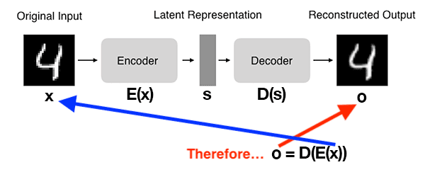
1. Encoder: Accepts the input data and compresses it into the latent-space. If we denote our input data as and the encoder as , then the output latent-space representation, , would be .
2. Decoder: The decoder is responsible for accepting the latent-space representation and then reconstructing the original input. If we denote the decoder function as and the output of the detector as , then we can represent the decoder as .

Using our mathematical notation, the entire training process of the autoencoder can be written as:

Figure 1 below demonstrates the basic architecture of an autoencoder:

Here you can see that:

1. We input a digit to the autoencoder.
2. The encoder subnetwork creates a latent representation of the digit. This latent representation is substantially smaller (in terms of dimensionality) than the input.
3. The decoder subnetwork then reconstructs the original digit from the latent representation.

You can thus think of an autoencoder as a network that reconstructs its input!

To train an autoencoder, we input our data, attempt to reconstruct it, and then minimize the mean squared error (or similar loss function).

Ideally, the output of the autoencoder will be near identical to the input.

An autoencoder reconstructs it’s input — so what’s the big deal?

At this point, some of you might be thinking:

Adrian, what’s the big deal here?

If the goal of an autoencoder is just to reconstruct the input, why even use the network in the first place?

If I wanted a copy of my input data, I could literally just copy it with a single function call.

Why on earth would I apply deep learning and go through the trouble of training a network?

This question, although a legitimate one, does indeed contain a large misconception regarding autoencoders.

Yes, during the training process, our goal is to train a network that can learn how to reconstruct our input data — but the true value of the autoencoder lives inside that latent-space representation.

Keep in mind that autoencoders compress our input data and, more to the point, when we train autoencoders, what we really care about is the encoder, , and the latent-space representation, .

The decoder, , is used to train the autoencoder end-to-end, but in practical applications, we often (but not always) care more about the encoder and the latent-space.

Later in this tutorial, we’ll be training an autoencoder on the MNIST dataset. The MNIST dataset consists of digits that are 28×28 pixels with a single channel, implying that each digit is represented by 28 x 28 = 784 values. The autoencoder we’ll be training here will be able to compress those digits into a vector of only 16 values — that’s a reduction of nearly 98%!

So what can we do if an input data point is compressed into such a small vector?

That’s where things get really interesting.

What are applications of autoencoders?

Autoencoders are typically used for:

• Dimensionality reduction (i.e., think PCA but more powerful/intelligent).
• Denoising (ex., removing noise and preprocessing images to improve OCR accuracy).
• Anomaly/outlier detection (ex., detecting mislabeled data points in a dataset or detecting when an input data point falls well outside our typical data distribution).

Outside of the computer vision field, you’ll see autoencoders applied to Natural Language Processing (NLP) and text comprehension problems, including understanding the semantic meaning of words, constructing word embeddings, and even text summarization.

How are autoencoders different from GANs?

If you’ve done any prior work with Generative Adversarial Networks (GANs), you might be wondering how autoencoders are different from GANs.

Both GANs and autoencoders are generative models; however, an autoencoder is essentially learning an identity function via compression.

The autoencoder will accept our input data, compress it down to the latent-space representation, and then attempt to reconstruct the input using just the latent-space vector.

Typically, the latent-space representation will have much fewer dimensions than the original input data.

GANs on the other hand:

1. Accept a low dimensional input.
2. Build a high dimensional space from it.
3. Generate the final output, which is not part of the original training data but ideally passes as such.

Furthermore, GANs have an evolving loss landscape, which autoencoders do not.

As a GAN is trained, the generative model generates “fake” images that are then mixed with actual “real” images — the discriminator model must then determine which images are “real” vs. “fake/generated”.

As the generative model becomes better and better at generating fake images that can fool the discriminator, the loss landscape evolves and changes (this is one of the reasons why training GANs is so damn hard).

While both GANs and autoencoders are generative models, most of their similarities end there.

Autoencoders cannot generate new, realistic data points that could be considered “passable” by humans. Instead, autoencoders are primarily used as a method to compress input data points into a latent-space representation. That latent-space representation can then be used for compression, denoising, anomaly detection, etc.

For more details on the differences between GANs and autoencoders, I suggest giving this thread on Quora a read.

Configuring your development environment

To follow along with today’s tutorial on autoencoders, you should use TensorFlow 2.0. I have two installation tutorials for TF 2.0 and associated packages to bring your development system up to speed:

• How to install TensorFlow 2.0 on Ubuntu (Ubuntu 18.04 OS; CPU and optional NVIDIA GPU)
• How to install TensorFlow 2.0 on macOS (Catalina and Mojave OSes)

Please note: PyImageSearch does not support Windows — refer to our FAQ.

Project structure

Be sure to grab the “Downloads” associated with the blog post. From there, extract the .zip and inspect the file/folder layout:

$ tree --dirsfirst
.
├── pyimagesearch
│   ├── __init__.py
│   └── convautoencoder.py
├── output.png
├── plot.png
└── train_conv_autoencoder.py

1 directory, 5 files

We will review two Python scripts today:

• convautoencoder.py: Contains the ConvAutoencoder class and build method required to assemble our neural network with tf.keras.
• train_conv_autoencoder.py: Trains a digits autoencoder on the MNIST dataset. Once the autoencoder is trained, we’ll loop over a number of output examples and write them to disk for later inspection.

Our training script results in both a plot.png figure and output.png image. The output image contains side-by-side samples of the original versus reconstructed image.

In the next section, we will implement our autoencoder with the high-level Keras API built into TensorFlow.

Implementing a convolutional autoencoder with Keras and TensorFlow

Before we can train an autoencoder, we first need to implement the autoencoder architecture itself.

To do so, we’ll be using Keras and TensorFlow.

My implementation loosely follows Francois Chollet’s own implementation of autoencoders on the official Keras blog. My primary contribution here is to go into a bit more detail regarding the implementation itself.

Open up the convautoencoder.py file in your project structure, and insert the following code:

# import the necessary packages
from tensorflow.keras.layers import BatchNormalization
from tensorflow.keras.layers import Conv2D
from tensorflow.keras.layers import Conv2DTranspose
from tensorflow.keras.layers import LeakyReLU
from tensorflow.keras.layers import Activation
from tensorflow.keras.layers import Flatten
from tensorflow.keras.layers import Dense
from tensorflow.keras.layers import Reshape
from tensorflow.keras.layers import Input
from tensorflow.keras.models import Model
from tensorflow.keras import backend as K
import numpy as np

class ConvAutoencoder:
	@staticmethod
	def build(width, height, depth, filters=(32, 64), latentDim=16):
		# initialize the input shape to be "channels last" along with
		# the channels dimension itself
		# channels dimension itself
		inputShape = (height, width, depth)
		chanDim = -1

We begin with a selection of imports from tf.keras and one from NumPy. If you don’t have TensorFlow 2.0 installed on your system, refer to the “Configuring your development environment” section above.

Our ConvAutoencoder class contains one static method, build, which accepts five parameters:

• width: Width of the input image in pixels.
• height: Height of the input image in pixels.
• depth: Number of channels (i.e., depth) of the input volume.
• filters: A tuple that contains the set of filters for convolution operations. By default, this parameter includes both 32 and 64 filters.
• latentDim: The number of neurons in our fully-connected (Dense) latent vector. By default, if this parameter is not passed, the value is set to 16.

From there, we initialize the inputShape and channel dimension (we assume “channels last” ordering).

We’re now ready to initialize our input and begin adding layers to our network:

		# define the input to the encoder
		inputs = Input(shape=inputShape)
		x = inputs

		# loop over the number of filters
		for f in filters:
			# apply a CONV => RELU => BN operation
			x = Conv2D(f, (3, 3), strides=2, padding="same")(x)
			x = LeakyReLU(alpha=0.2)(x)
			x = BatchNormalization(axis=chanDim)(x)

		# flatten the network and then construct our latent vector
		volumeSize = K.int_shape(x)
		x = Flatten()(x)
		latent = Dense(latentDim)(x)

		# build the encoder model
		encoder = Model(inputs, latent, name="encoder")

Lines 25 and 26 define the input to the encoder.

With our inputs ready, we go loop over the number of filters and add our sets of CONV=>LeakyReLU=>BN layers (Lines 29-33).

Next, we flatten the network and construct our latent vector (Lines 36-38) — this is our actual latent-space representation (i.e., the “compressed” data representation).

We then build our encoder model (Line 41).

If we were to do a print(encoder.summary()) of the encoder, assuming 28×28 single channel images (depth=1) and filters=(32, 64) and latentDim=16, we would have the following:

Model: "encoder"
_________________________________________________________________
Layer (type)                 Output Shape              Param #
=================================================================
input_1 (InputLayer)         [(None, 28, 28, 1)]       0
_________________________________________________________________
conv2d (Conv2D)              (None, 14, 14, 32)        320
_________________________________________________________________
leaky_re_lu (LeakyReLU)      (None, 14, 14, 32)        0
_________________________________________________________________
batch_normalization (BatchNo (None, 14, 14, 32)        128
_________________________________________________________________
conv2d_1 (Conv2D)            (None, 7, 7, 64)          18496
_________________________________________________________________
leaky_re_lu_1 (LeakyReLU)    (None, 7, 7, 64)          0
_________________________________________________________________
batch_normalization_1 (Batch (None, 7, 7, 64)          256
_________________________________________________________________
flatten (Flatten)            (None, 3136)              0
_________________________________________________________________
dense (Dense)                (None, 16)                50192
=================================================================
Total params: 69,392
Trainable params: 69,200
Non-trainable params: 192
_________________________________________________________________

Here we can observe that:

• Our encoder begins by accepting a 28x28x1 input volume.
• We then apply two rounds of CONV=>RELU=>BN, each with 3×3 strided convolution. The strided convolution allows us to reduce the spatial dimensions of our volumes.
• After applying our final batch normalization, we end up with a 7x7x64 volume, which is flattened into a 3136-dim vector.
• Our fully-connected layer (i.e., the Dense layer) serves our as our latent-space representation.

Next, let’s learn how the decoder model can take this latent-space representation and reconstruct the original input image:

		# start building the decoder model which will accept the
		# output of the encoder as its inputs
		latentInputs = Input(shape=(latentDim,))
		x = Dense(np.prod(volumeSize[1:]))(latentInputs)
		x = Reshape((volumeSize[1], volumeSize[2], volumeSize[3]))(x)

		# loop over our number of filters again, but this time in
		# reverse order
		for f in filters[::-1]:
			# apply a CONV_TRANSPOSE => RELU => BN operation
			x = Conv2DTranspose(f, (3, 3), strides=2,
				padding="same")(x)
			x = LeakyReLU(alpha=0.2)(x)
			x = BatchNormalization(axis=chanDim)(x)

To start building the decoder model, we:

• Construct the input to the decoder model based on the latentDim. (Lines 45 and 46).
• Accept the 1D latentDim vector and turn it into a 2D volume so that we can start applying convolution (Line 47).
• Loop over the number of filters, this time in reverse order while applying a CONV_TRANSPOSE => RELU => BN operation (Lines 51-56).

Transposed convolution is used to increase the spatial dimensions (i.e., width and height) of the volume.

Let’s finish creating our autoencoder:

		# apply a single CONV_TRANSPOSE layer used to recover the
		# original depth of the image
		x = Conv2DTranspose(depth, (3, 3), padding="same")(x)
		outputs = Activation("sigmoid")(x)

		# build the decoder model
		decoder = Model(latentInputs, outputs, name="decoder")

		# our autoencoder is the encoder + decoder
		autoencoder = Model(inputs, decoder(encoder(inputs)),
			name="autoencoder")

		# return a 3-tuple of the encoder, decoder, and autoencoder
		return (encoder, decoder, autoencoder)

Wrapping up, we:

• Apply a final CONV_TRANSPOSE layer used to recover the original channel depth of the image (1 channel for single channel/grayscale images or 3 channels for RGB images) on Line 60.
• Apply a sigmoid activation function (Line 61).
• Build the decoder model, and add it with the encoder to the autoencoder (Lines 64-68). The autoencoder becomes the encoder + decoder.
• Return a 3-tuple of the encoder, decoder, and autoencoder.

If we were to complete a print(decoder.summary()) operation here, we would have the following:

Model: "decoder"
_________________________________________________________________
Layer (type)                 Output Shape              Param #
=================================================================
input_2 (InputLayer)         [(None, 16)]              0
_________________________________________________________________
dense_1 (Dense)              (None, 3136)              53312
_________________________________________________________________
reshape (Reshape)            (None, 7, 7, 64)          0
_________________________________________________________________
conv2d_transpose (Conv2DTran (None, 14, 14, 64)        36928
_________________________________________________________________
leaky_re_lu_2 (LeakyReLU)    (None, 14, 14, 64)        0
_________________________________________________________________
batch_normalization_2 (Batch (None, 14, 14, 64)        256
_________________________________________________________________
conv2d_transpose_1 (Conv2DTr (None, 28, 28, 32)        18464
_________________________________________________________________
leaky_re_lu_3 (LeakyReLU)    (None, 28, 28, 32)        0
_________________________________________________________________
batch_normalization_3 (Batch (None, 28, 28, 32)        128
_________________________________________________________________
conv2d_transpose_2 (Conv2DTr (None, 28, 28, 1)         289
_________________________________________________________________
activation (Activation)      (None, 28, 28, 1)         0
=================================================================
Total params: 109,377
Trainable params: 109,185
Non-trainable params: 192
_________________________________________________________________

The decoder accepts our 16-dim latent representation from the encoder and then builds a new fully-connected layer of 3136-dim, which is the product of 7 x 7 x 64 = 3136.

Using our new 3136-dim FC layer, we reshape it into a 3D volume of 7 x 7 x 64. From there we can start applying our CONV_TRANSPOSE=>RELU=>BN operation. Unlike standard strided convolution, which is used to decrease volume size, our transposed convolution is used to increase volume size.

Finally, a transposed convolution layer is applied to recover the original channel depth of the image. Since our images are grayscale, we learn a single filter, the output of which is a 28 x 28 x 1 volume (i.e., the dimensions of the original MNIST digit images).

A print(autoencoder.summary()) operation shows the composed nature of the encoder and decoder:

Model: "autoencoder"
_________________________________________________________________
Layer (type)                 Output Shape              Param #
=================================================================
input_1 (InputLayer)         [(None, 28, 28, 1)]       0
_________________________________________________________________
encoder (Model)              (None, 16)                69392
_________________________________________________________________
decoder (Model)              (None, 28, 28, 1)         109377
=================================================================
Total params: 178,769
Trainable params: 178,385
Non-trainable params: 384
_________________________________________________________________

The input to our encoder is the original 28 x 28 x 1 images from the MNIST dataset. Our encoder then learns a 16-dim latent-space representation of the data, after which the decoder reconstructs the original 28 x 28 x 1 images.

In the next section, we will develop our script to train our autoencoder.

Creating the convolutional autoencoder training script

With our autoencoder architecture implemented, let’s move on to the training script.

Open up the train_conv_autoencoder.py in your project directory structure, and insert the following code:

# set the matplotlib backend so figures can be saved in the background
import matplotlib
matplotlib.use("Agg")

# import the necessary packages
from pyimagesearch.convautoencoder import ConvAutoencoder
from tensorflow.keras.optimizers import Adam
from tensorflow.keras.datasets import mnist
import matplotlib.pyplot as plt
import numpy as np
import argparse
import cv2

# construct the argument parse and parse the arguments
ap = argparse.ArgumentParser()
ap.add_argument("-s", "--samples", type=int, default=8,
	help="# number of samples to visualize when decoding")
ap.add_argument("-o", "--output", type=str, default="output.png",
	help="path to output visualization file")
ap.add_argument("-p", "--plot", type=str, default="plot.png",
	help="path to output plot file")
args = vars(ap.parse_args())

On Lines 2-12, we handle our imports. We’ll use the "Agg" backend of matplotlib so that we can export our training plot to disk.

We need our custom ConvAutoencoder architecture class which we implemented in the previous section.

We will use the Adam optimizer as we train on the MNIST benchmarking dataset. For visualization, we’ll employ OpenCV.

Next, we’ll parse three command line arguments, all of which are optional:

• --samples: The number of output samples for visualization. By default this value is set to 8.
• --output: The path the output visualization image. We’ll name our visualization output.png by default
• --plot: The path to our matplotlib output plot. A default of plot.png is assigned if this argument is not provided in the terminal.

Now we’ll set a couple hyperparameters and preprocess our MNIST dataset:

# initialize the number of epochs to train for and batch size
EPOCHS = 25
BS = 32

# load the MNIST dataset
print("[INFO] loading MNIST dataset...")
((trainX, _), (testX, _)) = mnist.load_data()

# add a channel dimension to every image in the dataset, then scale
# the pixel intensities to the range [0, 1]
trainX = np.expand_dims(trainX, axis=-1)
testX = np.expand_dims(testX, axis=-1)
trainX = trainX.astype("float32") / 255.0
testX = testX.astype("float32") / 255.0

Lines 25 and 26 initialize the batch size and number of training epochs.

From there, we’ll work with our MNIST dataset. TensorFlow/Keras has a handy load_data method that we can call on mnist to grab the data (Line 30). From there, Lines 34-37 (1) add a channel dimension to every image in the dataset and (2) scale the pixel intensities to the range [0, 1].

We’re now ready to build and train our autoencoder:

# construct our convolutional autoencoder
print("[INFO] building autoencoder...")
(encoder, decoder, autoencoder) = ConvAutoencoder.build(28, 28, 1)
opt = Adam(lr=1e-3)
autoencoder.compile(loss="mse", optimizer=opt)

# train the convolutional autoencoder
H = autoencoder.fit(
	trainX, trainX,
	validation_data=(testX, testX),
	epochs=EPOCHS,
	batch_size=BS)

To build the convolutional autoencoder, we call the build method on our ConvAutoencoder class and pass the necessary arguments (Line 41). Recall that this results in the (encoder, decoder, autoencoder) tuple — going forward in this script, we only need the autoencoder for training and predictions.

We initialize our Adam optimizer with an initial learning rate of 1e-3 and go ahead and compile it with mean-squared error loss (Lines 42 and 43).

From there, we fit (train) our autoencoder on the MNIST data (Lines 46-50).

Let’s go ahead and plot our training history:

# construct a plot that plots and saves the training history
N = np.arange(0, EPOCHS)
plt.style.use("ggplot")
plt.figure()
plt.plot(N, H.history["loss"], label="train_loss")
plt.plot(N, H.history["val_loss"], label="val_loss")
plt.title("Training Loss and Accuracy")
plt.xlabel("Epoch #")
plt.ylabel("Loss/Accuracy")
plt.legend(loc="lower left")
plt.savefig(args["plot"])

And from there, we’ll make predictions on our testing set:

# use the convolutional autoencoder to make predictions on the
# testing images, then initialize our list of output images
print("[INFO] making predictions...")
decoded = autoencoder.predict(testX)
outputs = None

# loop over our number of output samples
for i in range(0, args["samples"]):
	# grab the original image and reconstructed image
	original = (testX[i] * 255).astype("uint8")
	recon = (decoded[i] * 255).astype("uint8")

	# stack the original and reconstructed image side-by-side
	output = np.hstack([original, recon])

	# if the outputs array is empty, initialize it as the current
	# side-by-side image display
	if outputs is None:
		outputs = output

	# otherwise, vertically stack the outputs
	else:
		outputs = np.vstack([outputs, output])

# save the outputs image to disk
cv2.imwrite(args["output"], outputs)

Line 67 makes predictions on the test set. We then loop over the number of --samples passed as a command line argument (Line 71) so that we can build our visualization. Inside the loop, we:

• Grab both the original and reconstructed images (Lines 73 and 74).
• Stack the pair of images side-by-side (Line 77).
• Stack the pairs vertically (Lines 81-86).
• Finally, we output the visualization image to disk (Line 89).

In the next section, we’ll see the results of our hard work.

Training the convolutional autoencoder with Keras and TensorFlow

We are now ready to see our autoencoder in action!

Make sure you use the “Downloads” section of this post to download the source code — from there you can execute the following command:

$ python train_conv_autoencoder.py
[INFO] loading MNIST dataset...
[INFO] building autoencoder...
Train on 60000 samples, validate on 10000 samples
Epoch 1/25
60000/60000 [==============================] - 68s 1ms/sample - loss: 0.0188 - val_loss: 0.0108
Epoch 2/25
60000/60000 [==============================] - 68s 1ms/sample - loss: 0.0104 - val_loss: 0.0096
Epoch 3/25
60000/60000 [==============================] - 68s 1ms/sample - loss: 0.0094 - val_loss: 0.0086
Epoch 4/25
60000/60000 [==============================] - 68s 1ms/sample - loss: 0.0088 - val_loss: 0.0086
Epoch 5/25
60000/60000 [==============================] - 68s 1ms/sample - loss: 0.0084 - val_loss: 0.0080
...
Epoch 20/25
60000/60000 [==============================] - 83s 1ms/sample - loss: 0.0067 - val_loss: 0.0069
Epoch 21/25
60000/60000 [==============================] - 83s 1ms/sample - loss: 0.0066 - val_loss: 0.0069
Epoch 22/25
60000/60000 [==============================] - 83s 1ms/sample - loss: 0.0066 - val_loss: 0.0068
Epoch 23/25
60000/60000 [==============================] - 83s 1ms/sample - loss: 0.0066 - val_loss: 0.0068
Epoch 24/25
60000/60000 [==============================] - 83s 1ms/sample - loss: 0.0065 - val_loss: 0.0067
Epoch 25/25
60000/60000 [==============================] - 83s 1ms/sample - loss: 0.0065 - val_loss: 0.0068
[INFO] making predictions...

As Figure 4 and the terminal output demonstrate, our training process was able to minimize the reconstruction loss of the autoencoder.

But how well did the autoencoder do at reconstructing the training data?

The answer is very good:

In Figure 5, on the left is our original image while the right is the reconstructed digit predicted by the autoencoder. As you can see, the digits are nearly indistinguishable from each other!

At this point, you may be thinking:

Great … so I can train a network to reconstruct my original image.

But you said that what really matters is the internal latent-space representation.

How can I access that representation, and how can I use it for denoising and anomaly/outlier detection?

Those are great questions — I’ll be addressing both in my next two tutorials here on PyImageSearch, so stay tuned!

What’s next?

This tutorial and the next two in this series admittedly discuss advanced applications of computer vision and deep learning.

If you don’t already know the fundamentals of deep learning, now would be a good time to learn them. To get a head start, I personally suggest you read my book, Deep Learning for Computer Vision with Python.

Inside the book, you will learn:

• Deep learning fundamentals and theory without unnecessary mathematical fluff. I present the basic equations and back them up with code walkthroughs that you can implement and easily understand. You don’t need a degree in advanced mathematics to understand this book.
• How to implement your own custom neural network architectures. Not only will you learn how to implement state-of-the-art architectures, including ResNet, SqueezeNet, etc., but you’ll also learn how to create your own custom CNNs.
• How to train CNNs on your own datasets. Most deep learning tutorials don’t teach you how to work with your own custom datasets. Mine do. You’ll be training CNNs on your own datasets in no time.
• Object detection (Faster R-CNNs, Single Shot Detectors, and RetinaNet) and instance segmentation (Mask R-CNN). Use these chapters to create your own custom object detectors and segmentation networks.

If you’re interested in learning more about the book, I’d be happy to send you a free PDF containing the Table of Contents and a few sample chapters. Simply click the button below:

Summary

In this tutorial, you learned the fundamentals of autoencoders.

Autoencoders are generative models that consist of an encoder and a decoder model. When trained, the encoder takes input data point and learns a latent-space representation of the data. This latent-space representation is a compressed representation of the data, allowing the model to represent it in far fewer parameters than the original data.

The decoder model then takes the latent-space representation and attempts to reconstruct the original data point from it. When trained end-to-end, the encoder and decoder function in a composed manner.

In practice, we use autoencoders for dimensionality reduction, compression, denoising, and anomaly detection.

After we understood the fundamentals, we implemented a convolutional autoencoder using Keras and TensorFlow.

In next week’s tutorial, we’ll learn how to use a convolutional autoencoder for denoising.

To download the source code to this post (and be notified when future tutorials are published here on PyImageSearch), just enter your email address in the form below!

Download the Source Code and FREE 17-page Resource Guide

Enter your email address below to get a .zip of the code and a FREE 17-page Resource Guide on Computer Vision, OpenCV, and Deep Learning. Inside you’ll find my hand-picked tutorials, books, courses, and libraries to help you master CV and DL!

Download the code!

Website

The post Autoencoders with Keras, TensorFlow, and Deep Learning appeared first on PyImageSearch.

In this tutorial, you will learn how to use autoencoders to denoise images using Keras, TensorFlow, and Deep Learning.

Today’s tutorial is part two in our three-part series on the applications of autoencoders:

1. Autoencoders with Keras, TensorFlow, and Deep Learning (last week’s tutorial)
2. Denoising autoenecoders with Keras, TensorFlow and Deep Learning (today’s tutorial)
3. Anomaly detection with Keras, TensorFlow, and Deep Learning (next week’s tutorial)

Last week you learned the fundamentals of autoencoders, including how to train your very first autoencoder using Keras and TensorFlow — however, the real-world application of that tutorial was admittedly a bit limited due to the fact that we needed to lay the groundwork.

Today, we’re going to take a deeper dive and learn how autoencoders can be used for denoising, also called “noise reduction,” which is the process of removing noise from a signal.

The term “noise” here could be:

• Produced by a faulty or poor quality image sensor
• Random variations in brightness or color
• Quantization noise
• Artifacts due to JPEG compression
• Image perturbations produced by an image scanner or threshold post-processing
• Poor paper quality (crinkles and folds) when trying to perform OCR

From the perspective of image processing and computer vision, you should think of noise as anything that could be removed by a really good pre-processing filter.

Our goal is to train an autoencoder to perform such pre-processing — we call such models denoising autoencoders.

To learn how to train a denoising autoencoder with Keras and TensorFlow, just keep reading!

Looking for the source code to this post?

Jump Right To The Downloads Section

Denoising autoencoders with Keras, TensorFlow, and Deep Learning

In the first part of this tutorial, we’ll discuss what denoising autoencoders are and why we may want to use them.

From there I’ll show you how to implement and train a denoising autoencoder using Keras and TensorFlow.

We’ll wrap up this tutorial by examining the results of our denoising autoencoder.

What are denoising autoencoders, and why would we use them?

Denoising autoencoders are an extension of simple autoencoders; however, it’s worth noting that denoising autoencoders were not originally meant to automatically denoise an image.

Instead, the denoising autoencoder procedure was invented to help:

• The hidden layers of the autoencoder learn more robust filters
• Reduce the risk of overfitting in the autoencoder
• Prevent the autoencoder from learning a simple identify function

In Vincent et al.’s 2008 ICML paper, Extracting and Composing Robust Features with Denoising Autoencoders, the authors found that they could improve the robustness of their internal layers (i.e., latent-space representation) by purposely introducing noise to their signal.

Noise was stochastically (i.e., randomly) added to the input data, and then the autoencoder was trained to recover the original, nonperturbed signal.

From an image processing standpoint, we can train an autoencoder to perform automatic image pre-processing for us.

A great example would be pre-processing an image to improve the accuracy of an optical character recognition (OCR) algorithm. If you’ve ever applied OCR before, you know how just a little bit of the wrong type of noise (ex., printer ink smudges, poor image quality during the scan, etc.) can dramatically hurt the performance of your OCR method. Using denoising autoencoders, we can automatically pre-process the image, improve the quality, and therefore increase the accuracy of the downstream OCR algorithm.

If you’re interested in learning more about denoising autoencoders, I would strongly encourage you to read this article as well Bengio and Delalleau’s paper, Justifying and Generalizing Contrastive Divergence.

For more information on denoising autoencoders for OCR-related preprocessing, take a look at this dataset on Kaggle.

Configuring your development environment

To follow along with today’s tutorial on autoencoders, you should use TensorFlow 2.0. I have two installation tutorials for TF 2.0 and associated packages to bring your development system up to speed:

• How to install TensorFlow 2.0 on Ubuntu (Ubuntu 18.04 OS; CPU and optional NVIDIA GPU)
• How to install TensorFlow 2.0 on macOS (Catalina and Mojave OSes)

Please note: PyImageSearch does not support Windows — refer to our FAQ.

Project structure

Go ahead and grab the .zip from the “Downloads” section of today’s tutorial. From there, extract the zip.

You’ll be presented with the following project layout:

$ tree --dirsfirst
.
├── pyimagesearch
│   ├── __init__.py
│   └── convautoencoder.py
├── output.png
├── plot.png
└── train_denoising_autoencoder.py

1 directory, 5 files

The pyimagesearch module contains the ConvAutoencoder class. We reviewed this class in our previous tutorial; however, we’ll briefly walk through it again today.

The heart of today’s tutorial is inside the train_denoising_autoencoder.py Python training script. This script is different from the previous tutorial in one main way:

We will purposely add noise to our MNIST training images using a random normal distribution centered at 0.5 with a standard deviation of 0.5.

The purpose of adding noise to our training data is so that our autoencoder can effectively remove noise from an input image (i.e., denoise).

Implementing our denoising autoencoder with Keras and TensorFlow

The denoising autoencoder we’ll be implementing today is essentially identical to the one we implemented in last week’s tutorial on autoencoder fundamentals.

We’ll review the model architecture here today as a matter of completeness, but make sure you refer to last week’s guide for more details.

With that said, open up the convautoencoder.py file in your project structure, and insert the following code:

# import the necessary packages
from tensorflow.keras.layers import BatchNormalization
from tensorflow.keras.layers import Conv2D
from tensorflow.keras.layers import Conv2DTranspose
from tensorflow.keras.layers import LeakyReLU
from tensorflow.keras.layers import Activation
from tensorflow.keras.layers import Flatten
from tensorflow.keras.layers import Dense
from tensorflow.keras.layers import Reshape
from tensorflow.keras.layers import Input
from tensorflow.keras.models import Model
from tensorflow.keras import backend as K
import numpy as np

class ConvAutoencoder:
	@staticmethod
	def build(width, height, depth, filters=(32, 64), latentDim=16):
		# initialize the input shape to be "channels last" along with
		# the channels dimension itself
		# channels dimension itself
		inputShape = (height, width, depth)
		chanDim = -1

		# define the input to the encoder
		inputs = Input(shape=inputShape)
		x = inputs

Imports include tf.keras and NumPy.

Our ConvAutoencoder class contains one static method, build which accepts five parameters:

• width: Width of the input image in pixels
• height: Heigh of the input image in pixels
• depth: Number of channels (i.e., depth) of the input volume
• filters: A tuple that contains the set of filters for convolution operations. By default, if this parameter is not provided by the caller, we’ll add two sets of CONV => RELU => BN with 32 and 64 filters
• latentDim: The number of neurons in our fully-connected (Dense) latent vector. By default, if this parameter is not passed, the value is set to 16

From there, we initialize the inputShape and define the Input to the encoder (Lines 25 and 26).

Let’s begin building our encoder’s filters:

		# loop over the number of filters
		for f in filters:
			# apply a CONV => RELU => BN operation
			x = Conv2D(f, (3, 3), strides=2, padding="same")(x)
			x = LeakyReLU(alpha=0.2)(x)
			x = BatchNormalization(axis=chanDim)(x)

		# flatten the network and then construct our latent vector
		volumeSize = K.int_shape(x)
		x = Flatten()(x)
		latent = Dense(latentDim)(x)

		# build the encoder model
		encoder = Model(inputs, latent, name="encoder")

Using Keras’ functional API, we go ahead and Loop over number of filters and add our sets of CONV => RELU => BN layers (Lines 29-33).

We then flatten the network and construct our latent vector (Lines 36-38). The latent-space representation is the compressed form of our data.

From there, we build the encoder portion of our autoencoder (Line 41).

Next, we’ll use our latent-space representation to reconstruct the original input image.

		# start building the decoder model which will accept the
		# output of the encoder as its inputs
		latentInputs = Input(shape=(latentDim,))
		x = Dense(np.prod(volumeSize[1:]))(latentInputs)
		x = Reshape((volumeSize[1], volumeSize[2], volumeSize[3]))(x)

		# loop over our number of filters again, but this time in
		# reverse order
		for f in filters[::-1]:
			# apply a CONV_TRANSPOSE => RELU => BN operation
			x = Conv2DTranspose(f, (3, 3), strides=2,
				padding="same")(x)
			x = LeakyReLU(alpha=0.2)(x)
			x = BatchNormalization(axis=chanDim)(x)

		# apply a single CONV_TRANSPOSE layer used to recover the
		# original depth of the image
		x = Conv2DTranspose(depth, (3, 3), padding="same")(x)
		outputs = Activation("sigmoid")(x)

		# build the decoder model
		decoder = Model(latentInputs, outputs, name="decoder")

		# our autoencoder is the encoder + decoder
		autoencoder = Model(inputs, decoder(encoder(inputs)),
			name="autoencoder")

		# return a 3-tuple of the encoder, decoder, and autoencoder
		return (encoder, decoder, autoencoder)

Here, we are taking the latent input and use a fully-connected layer to reshape it into a 3D volume (i.e., the image data).

We loop over our filters again, but in reverse order, applying CONV_TRANSPOSE => RELU => BN layers where the CONV_TRANSPOSE layer’s purpose is to increase the volume size.

Finally, we build the decoder model and construct the autoencoder. Remember, the concept of an autoencoder — discussed last week — consists of both the encoder and decoder components.

Implementing the denoising autoencoder training script

Let’s now implement the training script used to:

1. Add stochastic noise to the MNIST dataset
2. Train a denoising autoencoder on the noisy dataset
3. Automatically recover the original digits from the noise

My implementation follows Francois Chollet’s own implementation of denoising autoencoders on the official Keras blog — my primary contribution here is to go into a bit more detail regarding the implementation itself.

Open up the train_denoising_autoencoder.py file, and insert the following code:

# set the matplotlib backend so figures can be saved in the background
import matplotlib
matplotlib.use("Agg")

# import the necessary packages
from pyimagesearch.convautoencoder import ConvAutoencoder
from tensorflow.keras.optimizers import Adam
from tensorflow.keras.datasets import mnist
import matplotlib.pyplot as plt
import numpy as np
import argparse
import cv2

# construct the argument parse and parse the arguments
ap = argparse.ArgumentParser()
ap.add_argument("-s", "--samples", type=int, default=8,
	help="# number of samples to visualize when decoding")
ap.add_argument("-o", "--output", type=str, default="output.png",
	help="path to output visualization file")
ap.add_argument("-p", "--plot", type=str, default="plot.png",
	help="path to output plot file")
args = vars(ap.parse_args())

On Lines 2-12 we handle our imports. We’ll use the "Agg" backend of matplotlib so that we can export our training plot to disk. Our custom ConvAutoencoder class implemented in the previous section contains the autoencoder architecture itself. Modeling after Chollet’s example, we will also use the Adam optimizer.

Our script accepts three optional command line arguments:

• --samples: The number of output samples for visualization. By default this value is set to 8.
• --output: The path to the output visualization image. We’ll name our visualization output.png by default.
• --plot: The path to our matplotlib output plot. A default of plot.png is assigned if this argument is not provided in the terminal.

Next, we initialize hyperparameters and preprocess our MNIST dataset:

# initialize the number of epochs to train for and batch size
EPOCHS = 25
BS = 32

# load the MNIST dataset
print("[INFO] loading MNIST dataset...")
((trainX, _), (testX, _)) = mnist.load_data()

# add a channel dimension to every image in the dataset, then scale
# the pixel intensities to the range [0, 1]
trainX = np.expand_dims(trainX, axis=-1)
testX = np.expand_dims(testX, axis=-1)
trainX = trainX.astype("float32") / 255.0
testX = testX.astype("float32") / 255.0

Our training epochs will be 25 and we’ll use a batch size of 32.

We go ahead and grab the MNIST dataset (Line 30) while Lines 34-37 (1) add a channel dimension to every image in the dataset, and (2) scale the pixel intensities to the range [0, 1].

At this point, we’ll deviate from last week’s tutorial:

# sample noise from a random normal distribution centered at 0.5 (since
# our images lie in the range [0, 1]) and a standard deviation of 0.5
trainNoise = np.random.normal(loc=0.5, scale=0.5, size=trainX.shape)
testNoise = np.random.normal(loc=0.5, scale=0.5, size=testX.shape)
trainXNoisy = np.clip(trainX + trainNoise, 0, 1)
testXNoisy = np.clip(testX + testNoise, 0, 1)

To add random noise to the MNIST digits, we use NumPy’s random normal distribution centered at 0.5 with a standard deviation of 0.5 (Lines 41-44).

The following figure shows an example of how our images look before (left) adding noise followed by after (right):

As you can see, our images are quite corrupted — recovering the original digit from the noise will require a powerful model.

Luckily, our denoising autoencoder will be up to the task:

# construct our convolutional autoencoder
print("[INFO] building autoencoder...")
(encoder, decoder, autoencoder) = ConvAutoencoder.build(28, 28, 1)
opt = Adam(lr=1e-3)
autoencoder.compile(loss="mse", optimizer=opt)

# train the convolutional autoencoder
H = autoencoder.fit(
	trainXNoisy, trainX,
	validation_data=(testXNoisy, testX),
	epochs=EPOCHS,
	batch_size=BS)

# construct a plot that plots and saves the training history
N = np.arange(0, EPOCHS)
plt.style.use("ggplot")
plt.figure()
plt.plot(N, H.history["loss"], label="train_loss")
plt.plot(N, H.history["val_loss"], label="val_loss")
plt.title("Training Loss and Accuracy")
plt.xlabel("Epoch #")
plt.ylabel("Loss/Accuracy")
plt.legend(loc="lower left")
plt.savefig(args["plot"])

Line 48 builds our denoising autoencoder, passing the necessary arguments. Using our Adam optimizer with an initial learning rate of 1e-3, we go ahead and compile the autoencoder with mean-squared error loss (Lines 49 and 50).

Training is launched via Lines 53-57. Using the training history data, H, Lines 60-69 plot the loss, saving the resulting figure to disk.

Let’s write a quick loop that will help us visualize the denoising autoencoder results:

# use the convolutional autoencoder to make predictions on the
# testing images, then initialize our list of output images
print("[INFO] making predictions...")
decoded = autoencoder.predict(testX)
outputs = None

# loop over our number of output samples
for i in range(0, args["samples"]):
	# grab the original image and reconstructed image
	original = (testXNoisy[i] * 255).astype("uint8")
	recon = (decoded[i] * 255).astype("uint8")

	# stack the original and reconstructed image side-by-side
	output = np.hstack([original, recon])

	# if the outputs array is empty, initialize it as the current
	# side-by-side image display
	if outputs is None:
		outputs = output

	# otherwise, vertically stack the outputs
	else:
		outputs = np.vstack([outputs, output])

# save the outputs image to disk
cv2.imwrite(args["output"], outputs)

We go ahead and use our trained autoencoder to remove the noise from the images in our testing set (Line 74).

We then grab N --samples worth of original and reconstructed data, and put together a visualization montage (Lines 78-93). Line 96 writes the visualization figure to disk for inspection.

Training the denoising autoencoder with Keras and TensorFlow

To train your denoising autoencoder, make sure you use the “Downloads” section of this tutorial to download the source code.

From there, open up a terminal and execute the following command:

$ python train_denoising_autoencoder.py --output output_denoising.png \
	--plot plot_denoising.png
[INFO] loading MNIST dataset...
[INFO] building autoencoder...
Train on 60000 samples, validate on 10000 samples
Epoch 1/25
60000/60000 [==============================] - 85s 1ms/sample - loss: 0.0285 - val_loss: 0.0191
Epoch 2/25
60000/60000 [==============================] - 83s 1ms/sample - loss: 0.0187 - val_loss: 0.0211
Epoch 3/25
60000/60000 [==============================] - 84s 1ms/sample - loss: 0.0177 - val_loss: 0.0174
Epoch 4/25
60000/60000 [==============================] - 84s 1ms/sample - loss: 0.0171 - val_loss: 0.0170
Epoch 5/25
60000/60000 [==============================] - 83s 1ms/sample - loss: 0.0167 - val_loss: 0.0177
...
Epoch 21/25
60000/60000 [==============================] - 67s 1ms/sample - loss: 0.0146 - val_loss: 0.0161
Epoch 22/25
60000/60000 [==============================] - 67s 1ms/sample - loss: 0.0145 - val_loss: 0.0164
Epoch 23/25
60000/60000 [==============================] - 67s 1ms/sample - loss: 0.0145 - val_loss: 0.0158
Epoch 24/25
60000/60000 [==============================] - 67s 1ms/sample - loss: 0.0144 - val_loss: 0.0155
Epoch 25/25
60000/60000 [==============================] - 66s 1ms/sample - loss: 0.0144 - val_loss: 0.0157
[INFO] making predictions...

Training the denoising autoencoder on my iMac Pro with a 3 GHz Intel Xeon W processor took ~32.20 minutes.

As Figure 3 shows, our training process was stable and shows no signs of overfitting.

Denoising autoencoder results

Our denoising autoencoder has been successfully trained, but how did it perform when removing the noise we added to the MNIST dataset?

To answer that question, take a look at Figure 4:

On the left we have the original MNIST digits that we added noise to while on the right we have the output of the denoising autoencoder — we can clearly see that the denoising autoencoder was able to recover the original signal (i.e., digit) from the image while removing the noise.

More advanced denosing autoencoders can be used to automatically pre-process images to facilitate better OCR accuracy.

What’s next?

The path I took as I entered the field of deep learning and worked my way up to becoming an expert was not straightforward.

It was a grueling process of reading academic papers (some good, some junk), trying to figure out what all the terms mean, and trying to implement deep learning architectures from scratch. I became frustrated with my failed attempts at implementation, spending hours and days searching on Google, hunting for deep learning tutorials.

Back then, there weren’t many deep learning tutorials to be found, and while I also had some books stacked on my desk, they were too heavy with mathematical notation that professors thought would actually be useful to the average student.

Let’s face it, these days most of us don’t want to implement gradient descent or backpropagation algorithms by hand. While it can be a great learning exercise if you plan to write a dissertation on an improvement to the algorithm, we just want to learn how to train models on custom data.

In the age of internet-content-clickbait shared on social media, don’t blindly follow poorly written blog posts from nonreputable sources that you stumble upon. While free can be good, ultimately you get what you pay for.

Ask yourself:

• Do you want to hop around learning in an ad hoc manner, risking getting lost in the mess of free content available all over the net?
• Or do you want to study with the linear path that my deep learning book presents, arming you with a solid foundation with which you can build upon to study more advanced techniques?

Don’t study the way I did. It can be a great way to learn, but it isn’t efficient, and too many people find themselves giving up.

Instead, grab my book, Deep Learning for Computer Vision with Python so you can study the right way.

I crafted my book so that it perfectly balances theory with implementation, ensuring you properly master:

• Deep learning fundamentals and theory without unnecessary mathematical fluff. I present the basic equations and back them up with code walkthroughs that you can implement and easily understand. You don’t need a degree in advanced mathematics to understand this book.
• How to implement your own custom neural network architectures. Not only will you learn how to implement state-of-the-art architectures, including ResNet, SqueezeNet, etc., but you’ll also learn how to create your own custom CNNs.
• How to train CNNs on your own datasets. Most deep learning tutorials don’t teach you how to work with your own custom datasets. Mine do. You’ll be training CNNs on your own datasets in no time.
• Object detection (Faster R-CNNs, Single Shot Detectors, and RetinaNet) and instance segmentation (Mask R-CNN). Use these chapters to create your own custom object detectors and segmentation networks.

If you’re interested in learning more about the book, I’d be happy to send you a free PDF containing the Table of Contents and a few sample chapters:

Summary

In this tutorial, you learned about denoising autoencoders, which, as the name suggests, are models that are used to remove noise from a signal.

In the context of computer vision, denoising autoencoders can be seen as very powerful filters that can be used for automatic pre-processing. For example, a denoising autoencoder could be used to automatically pre-process an image, improving its quality for an OCR algorithm and thereby increasing OCR accuracy.

To demonstrate a denoising autoencoder in action, we added noise to the MNIST dataset, greatly degrading the image quality to the point where any model would struggle to correctly classify the digit in the image. Using our denoising autoencoder, we were able to remove the noise from the image, recovering the original signal (i.e., the digit).

In next week’s tutorial, you’ll learn about another real-world application of autoencoders — anomaly and outlier detection.

To download the source code to this post (and be notified when future tutorials are published here on PyImageSearch), just enter your email address in the form below!

Download the Source Code and FREE 17-page Resource Guide

Enter your email address below to get a .zip of the code and a FREE 17-page Resource Guide on Computer Vision, OpenCV, and Deep Learning. Inside you’ll find my hand-picked tutorials, books, courses, and libraries to help you master CV and DL!

Download the code!

Website

The post Denoising autoencoders with Keras, TensorFlow, and Deep Learning appeared first on PyImageSearch.

In this tutorial, you will learn how to perform anomaly and outlier detection using autoencoders, Keras, and TensorFlow.

Back in January, I showed you how to use standard machine learning models to perform anomaly detection and outlier detection in image datasets.

Our approach worked well enough, but it begged the question:

Could deep learning be used to improve the accuracy of our anomaly detector?

To answer such a question would require us to dive further down the rabbit hole and answer questions such as:

• What model architecture should we use?
• Are some deep neural network architectures better than others for anomaly/outlier detection?
• How do we handle the class imbalance problem?
• What if we wanted to train an unsupervised anomaly detector?

This tutorial addresses all of these questions, and by the end of it, you’ll be able to perform anomaly detection in your own image datasets using deep learning.

To learn how to perform anomaly detection with Keras, TensorFlow, and Deep Learning, just keep reading!

Looking for the source code to this post?

Jump Right To The Downloads Section

Anomaly detection with Keras, TensorFlow, and Deep Learning

In the first part of this tutorial, we’ll discuss anomaly detection, including:

• What makes anomaly detection so challenging
• Why traditional deep learning methods are not sufficient for anomaly/outlier detection
• How autoencoders can be used for anomaly detection

From there, we’ll implement an autoencoder architecture that can be used for anomaly detection using Keras and TensorFlow. We’ll then train our autoencoder model in an unsupervised fashion.

Once the autoencoder is trained, I’ll show you how you can use the autoencoder to identify outliers/anomalies in both your training/testing set as well as in new images that are not part of your dataset splits.

What is anomaly detection?

To quote my intro to anomaly detection tutorial:

Anomalies are defined as events that deviate from the standard, happen rarely, and don’t follow the rest of the “pattern.”

Examples of anomalies include:

• Large dips and spikes in the stock market due to world events
• Defective items in a factory/on a conveyor belt
• Contaminated samples in a lab

Depending on your exact use case and application, anomalies only typically occur 0.001-1% of the time — that’s an incredibly small fraction of the time.

The problem is only compounded by the fact that there is a massive imbalance in our class labels.

By definition, anomalies will rarely occur, so the majority of our data points will be of valid events.

To detect anomalies, machine learning researchers have created algorithms such as Isolation Forests, One-class SVMs, Elliptic Envelopes, and Local Outlier Factor to help detect such events; however, all of these methods are rooted in traditional machine learning.

What about deep learning?

Can deep learning be used for anomaly detection as well?

The answer is yes — but you need to frame the problem correctly.

How can deep learning and autoencoders be used for anomaly detection?

As I discussed in my intro to autoencoder tutorial, autoencoders are a type of unsupervised neural network that can:

1. Accept an input set of data
2. Internally compress the data into a latent-space representation
3. Reconstruct the input data from the latent representation

To accomplish this task, an autoencoder uses two components: an encoder and a decoder.

The encoder accepts the input data and compresses it into the latent-space representation. The decoder then attempts to reconstruct the input data from the latent space.

When trained in an end-to-end fashion, the hidden layers of the network learn filters that are robust and even capable of denoising the input data.

However, what makes autoencoders so special from an anomaly detection perspective is the reconstruction loss. When we train an autoencoder, we typically measure the mean-squared-error (MSE) between:

1. The input image
2. The reconstructed image from the autoencoder

The lower the loss, the better a job the autoencoder is doing at reconstructing the image.

Let’s now suppose that we trained an autoencoder on the entirety of the MNIST dataset:

We then present the autoencoder with a digit and tell it to reconstruct it:

We would expect the autoencoder to do a really good job at reconstructing the digit, as that is exactly what the autoencoder was trained to do — and if we were to look at the MSE between the input image and the reconstructed image, we would find that it’s quite low.

Let’s now suppose we presented our autoencoder with a photo of an elephant and asked it to reconstruct it:

Since the autoencoder has never seen an elephant before, and more to the point, was never trained to reconstruct an elephant, our MSE will be very high.

If the MSE of the reconstruction is high, then we likely have an outlier.

Alon Agmon does a great job explaining this concept in more detail in this article.

Configuring your development environment

To follow along with today’s tutorial on anomaly detection, I recommend you use TensorFlow 2.0.

To configure your system and install TensorFlow 2.0, you can follow either my Ubuntu or macOS guide:

• How to install TensorFlow 2.0 on Ubuntu (Ubuntu 18.04 OS; CPU and optional NVIDIA GPU)
• How to install TensorFlow 2.0 on macOS (Catalina and Mojave OSes)

Please note: PyImageSearch does not support Windows — refer to our FAQ.

Project structure

Go ahead and grab the code from the “Downloads” section of this post. Once you’ve unzipped the project, you’ll be presented with the following structure:

$ tree --dirsfirst
.
├── output
│   ├── autoencoder.model
│   └── images.pickle
├── pyimagesearch
│   ├── __init__.py
│   └── convautoencoder.py
├── find_anomalies.py
├── plot.png
├── recon_vis.png
└── train_unsupervised_autoencoder.py

2 directories, 8 files

Our convautoencoder.py file contains the ConvAutoencoder class which is responsible for building a Keras/TensorFlow autoencoder implementation.

We will train an autoencoder with unlabeled data inside train_unsupervised_autoencoder.py, resulting in the following outputs:

• autoencoder.model: The serialized, trained autoencoder model.
• images.pickle: A serialized set of unlabeled images for us to find anomalies in.
• plot.png: A plot consisting of our training loss curves.
• recon_vis.png: A visualization figure that compares samples of ground-truth digit images versus each reconstructed image.

From there, we will develop an anomaly detector inside find_anomalies.py and apply our autoencoder to reconstruct data and find anomalies.

Implementing our autoencoder for anomaly detection with Keras and TensorFlow

The first step to anomaly detection with deep learning is to implement our autoencoder script.

Our convolutional autoencoder implementation is identical to the ones from our introduction to autoencoders post as well as our denoising autoencoders tutorial; however, we’ll review it here as a matter of completeness — if you want additional details on autoencoders, be sure to refer to those posts.

Open up convautoencoder.py and inspect it:

# import the necessary packages
from tensorflow.keras.layers import BatchNormalization
from tensorflow.keras.layers import Conv2D
from tensorflow.keras.layers import Conv2DTranspose
from tensorflow.keras.layers import LeakyReLU
from tensorflow.keras.layers import Activation
from tensorflow.keras.layers import Flatten
from tensorflow.keras.layers import Dense
from tensorflow.keras.layers import Reshape
from tensorflow.keras.layers import Input
from tensorflow.keras.models import Model
from tensorflow.keras import backend as K
import numpy as np

class ConvAutoencoder:
	@staticmethod
	def build(width, height, depth, filters=(32, 64), latentDim=16):
		# initialize the input shape to be "channels last" along with
		# the channels dimension itself
		# channels dimension itself
		inputShape = (height, width, depth)
		chanDim = -1

		# define the input to the encoder
		inputs = Input(shape=inputShape)
		x = inputs

		# loop over the number of filters
		for f in filters:
			# apply a CONV => RELU => BN operation
			x = Conv2D(f, (3, 3), strides=2, padding="same")(x)
			x = LeakyReLU(alpha=0.2)(x)
			x = BatchNormalization(axis=chanDim)(x)

		# flatten the network and then construct our latent vector
		volumeSize = K.int_shape(x)
		x = Flatten()(x)
		latent = Dense(latentDim)(x)

		# build the encoder model
		encoder = Model(inputs, latent, name="encoder")

Imports include tf.keras and NumPy.

Our ConvAutoencoder class contains one static method, build, which accepts five parameters:

1. width: Width of the input images.
2. height: Height of the input images.
3. depth: Number of channels in the images.
4. filters: Number of filters the encoder and decoder will learn, respectively
5. latentDim: Dimensionality of the latent-space representation.

The Input is then defined for the encoder at which point we use Keras’ functional API to loop over our filters and add our sets of CONV => LeakyReLU => BN layers.

We then flatten the network and construct our latent vector. The latent-space representation is the compressed form of our data.

In the above code block we used the encoder portion of our autoencoder to construct our latent-space representation — this same representation will now be used to reconstruct the original input image:

		# start building the decoder model which will accept the
		# output of the encoder as its inputs
		latentInputs = Input(shape=(latentDim,))
		x = Dense(np.prod(volumeSize[1:]))(latentInputs)
		x = Reshape((volumeSize[1], volumeSize[2], volumeSize[3]))(x)

		# loop over our number of filters again, but this time in
		# reverse order
		for f in filters[::-1]:
			# apply a CONV_TRANSPOSE => RELU => BN operation
			x = Conv2DTranspose(f, (3, 3), strides=2,
				padding="same")(x)
			x = LeakyReLU(alpha=0.2)(x)
			x = BatchNormalization(axis=chanDim)(x)

		# apply a single CONV_TRANSPOSE layer used to recover the
		# original depth of the image
		x = Conv2DTranspose(depth, (3, 3), padding="same")(x)
		outputs = Activation("sigmoid")(x)

		# build the decoder model
		decoder = Model(latentInputs, outputs, name="decoder")

		# our autoencoder is the encoder + decoder
		autoencoder = Model(inputs, decoder(encoder(inputs)),
			name="autoencoder")

		# return a 3-tuple of the encoder, decoder, and autoencoder
		return (encoder, decoder, autoencoder)

Here, we are take the latent input and use a fully-connected layer to reshape it into a 3D volume (i.e., the image data).

We loop over our filters once again, but in reverse order, applying a series of CONV_TRANSPOSE => RELU => BN layers. The CONV_TRANSPOSE layer’s purpose is to increase the volume size back to the original image spatial dimensions.

Finally, we build the decoder model and construct the autoencoder. Recall that an autoencoder consists of both the encoder and decoder components. We then return a 3-tuple of the encoder, decoder, and autoencoder.

Again, if you need further details on the implementation of our autoencoder, be sure to review the aforementioned tutorials.

Implementing the anomaly detection training script

With our autoencoder implemented, we are now ready to move on to our training script.

Open up the train_unsupervised_autoencoder.py file in your project directory, and insert the following code:

# set the matplotlib backend so figures can be saved in the background
import matplotlib
matplotlib.use("Agg")

# import the necessary packages
from pyimagesearch.convautoencoder import ConvAutoencoder
from tensorflow.keras.optimizers import Adam
from tensorflow.keras.datasets import mnist
from sklearn.model_selection import train_test_split
import matplotlib.pyplot as plt
import numpy as np
import argparse
import random
import pickle
import cv2

Imports include our implementation of ConvAutoencoder, the mnist dataset, and a few imports from TensorFlow, scikit-learn, and OpenCV.

Given that we’re performing unsupervised learning, next we’ll define a function to build an unsupervised dataset:

def build_unsupervised_dataset(data, labels, validLabel=1,
	anomalyLabel=3, contam=0.01, seed=42):
	# grab all indexes of the supplied class label that are *truly*
	# that particular label, then grab the indexes of the image
	# labels that will serve as our "anomalies"
	validIdxs = np.where(labels == validLabel)[0]
	anomalyIdxs = np.where(labels == anomalyLabel)[0]

	# randomly shuffle both sets of indexes
	random.shuffle(validIdxs)
	random.shuffle(anomalyIdxs)

	# compute the total number of anomaly data points to select
	i = int(len(validIdxs) * contam)
	anomalyIdxs = anomalyIdxs[:i]

	# use NumPy array indexing to extract both the valid images and
	# "anomlay" images
	validImages = data[validIdxs]
	anomalyImages = data[anomalyIdxs]

	# stack the valid images and anomaly images together to form a
	# single data matrix and then shuffle the rows
	images = np.vstack([validImages, anomalyImages])
	np.random.seed(seed)
	np.random.shuffle(images)

	# return the set of images
	return images

Our build_supervised_dataset function accepts a labeled dataset (i.e., for supervised learning) and turns it into an unlabeled dataset (i.e., for unsupervised learning).

The function accepts a set of input data and labels, including valid label and anomaly label.

Given that our validLabel=1 by default, only MNIST numeral ones are selected; however, we’ll also contaminate our dataset with a set of numeral three images (validLabel=3).

The contam percentage is used to help us sample and select anomaly datapoints.

From our set of labels (and using the valid label), we generate a list of validIdxs (Line 22). The exact same process is applied to grab anomalyIdxs (Line 23). We then proceed to randomly shuffle the indices (Lines 26 and 27).

Given our anomaly contamination percentage, we reduce our set of anomalyIdxs (Lines 30 and 31).

Lines 35 and 36 then build two sets of images: (1) valid images and (2) anomaly images.

Each of these lists is stacked to form a single data matrix and then shuffled and returned (Lines 40-45). Notice that the labels have been intentionally discarded, effectively making our dataset ready for unsupervised learning.

Our next function will help us visualize predictions made by our unsupervised autoencoder:

def visualize_predictions(decoded, gt, samples=10):
	# initialize our list of output images
	outputs = None

	# loop over our number of output samples
	for i in range(0, samples):
		# grab the original image and reconstructed image
		original = (gt[i] * 255).astype("uint8")
		recon = (decoded[i] * 255).astype("uint8")

		# stack the original and reconstructed image side-by-side
		output = np.hstack([original, recon])

		# if the outputs array is empty, initialize it as the current
		# side-by-side image display
		if outputs is None:
			outputs = output

		# otherwise, vertically stack the outputs
		else:
			outputs = np.vstack([outputs, output])

	# return the output images
	return outputs

The visualize_predictions function is a helper method used to visualize the input images to our autoencoder as well as their corresponding output reconstructions. Both the original and reconstructed (recon) images will be arranged side-by-side and stacked vertically according to the number of samples parameter. This code should look familiar if you read either my introduction to autoencoders guide or denoising autoencoder tutorial.

Now that we’ve defined our imports and necessary functions, we’ll go ahead and parse our command line arguments:

# construct the argument parse and parse the arguments
ap = argparse.ArgumentParser()
ap.add_argument("-d", "--dataset", type=str, required=True,
	help="path to output dataset file")
ap.add_argument("-m", "--model", type=str, required=True,
	help="path to output trained autoencoder")
ap.add_argument("-v", "--vis", type=str, default="recon_vis.png",
	help="path to output reconstruction visualization file")
ap.add_argument("-p", "--plot", type=str, default="plot.png",
	help="path to output plot file")
args = vars(ap.parse_args())

Our function accepts four command line arguments, all of which are output file paths:

• --dataset: Defines the path to our output dataset file
• --model: Specifies the path to our output trained autoencoder
• --vis: An optional argument that specifies the output visualization file path. By default, I’ve named this file recon_vis.png; however, you are welcome to override it with a different path and filename
• --plot: Optionally indicates the path to our output training history plot. By default, the plot will be named plot.png in the current working directory

We’re now ready to prepare our data for training:

# initialize the number of epochs to train for, initial learning rate,
# and batch size
EPOCHS = 20
INIT_LR = 1e-3
BS = 32

# load the MNIST dataset
print("[INFO] loading MNIST dataset...")
((trainX, trainY), (testX, testY)) = mnist.load_data()

# build our unsupervised dataset of images with a small amount of
# contamination (i.e., anomalies) added into it
print("[INFO] creating unsupervised dataset...")
images = build_unsupervised_dataset(trainX, trainY, validLabel=1,
	anomalyLabel=3, contam=0.01)

# add a channel dimension to every image in the dataset, then scale
# the pixel intensities to the range [0, 1]
images = np.expand_dims(images, axis=-1)
images = images.astype("float32") / 255.0

# construct the training and testing split
(trainX, testX) = train_test_split(images, test_size=0.2,
	random_state=42)

First, we initialize three hyperparameters: (1) the number of training epochs, (2) the initial learning rate, and (3) our batch size (Lines 86-88).

Line 92 loads MNIST while Lines 97 and 98 build our unsupervised dataset with 1% contamination (i.e., anomalies) added into it.

From here forward, our dataset does not have labels, and our autoencoder will attempt to learn patterns without prior knowledge of what the data is.

Now that we’ve built out unsupervised dataset, it consists of 99% numeral ones and 1% numeral threes (i.e., anomalies/outliers).

From there, we preprocess our dataset by adding a channel dimension and scaling pixel intensities to the range [0, 1] (Lines 102 and 103).

Using scikit-learn’s convenience function, we then split data into 80% training and 20% testing sets (Lines 106 and 107).

Our data is ready to go, so let’s build our autoencoder and train it:

# construct our convolutional autoencoder
print("[INFO] building autoencoder...")
(encoder, decoder, autoencoder) = ConvAutoencoder.build(28, 28, 1)
opt = Adam(lr=INIT_LR, decay=INIT_LR / EPOCHS)
autoencoder.compile(loss="mse", optimizer=opt)

# train the convolutional autoencoder
H = autoencoder.fit(
	trainX, trainX,
	validation_data=(testX, testX),
	epochs=EPOCHS,
	batch_size=BS)

# use the convolutional autoencoder to make predictions on the
# testing images, construct the visualization, and then save it
# to disk
print("[INFO] making predictions...")
decoded = autoencoder.predict(testX)
vis = visualize_predictions(decoded, testX)
cv2.imwrite(args["vis"], vis)

We construct our autoencoder with the Adam optimizer and compile it with mean-squared-error loss (Lines 111-113).

Lines 116-120 launch the training procedure with TensorFlow/Keras. Our autoencoder will attempt to learn how to reconstruct the original input images. Images that cannot be easily reconstructed will have a large loss value.

Once training is complete, we’ll need a way to evaluate and visually inspect our results. Luckily, we have our visualize_predictions convenience function in our back pocket. Lines 126-128 make predictions on the test set, build a visualization image from the results, and write the output image to disk.

From here, we’ll wrap up:

# construct a plot that plots and saves the training history
N = np.arange(0, EPOCHS)
plt.style.use("ggplot")
plt.figure()
plt.plot(N, H.history["loss"], label="train_loss")
plt.plot(N, H.history["val_loss"], label="val_loss")
plt.title("Training Loss")
plt.xlabel("Epoch #")
plt.ylabel("Loss")
plt.legend(loc="lower left")
plt.savefig(args["plot"])

# serialize the image data to disk
print("[INFO] saving image data...")
f = open(args["dataset"], "wb")
f.write(pickle.dumps(images))
f.close()

# serialize the autoencoder model to disk
print("[INFO] saving autoencoder...")
autoencoder.save(args["model"], save_format="h5")

To close out, we:

• Plot our training history loss curves and export the resulting plot to disk (Lines 131-140)
• Serialize our unsupervised, sampled MNIST dataset to disk as a Python pickle file so that we can use it to find anomalies in the find_anomalies.py script (Lines 144-146)
• Save our trained autoencoder (Line 150)

Fantastic job developing the unsupervised autoencoder training script.

Training our anomaly detector using Keras and TensorFlow

To train our anomaly detector, make sure you use the “Downloads” section of this tutorial to download the source code.

From there, fire up a terminal and execute the following command:

$ python train_unsupervised_autoencoder.py \
	--dataset output/images.pickle \
	--model output/autoencoder.model
[INFO] loading MNIST dataset...
[INFO] creating unsupervised dataset...
[INFO] building autoencoder...
Train on 5447 samples, validate on 1362 samples
Epoch 1/20
5447/5447 [==============================] - 7s 1ms/sample - loss: 0.0421 - val_loss: 0.0405
Epoch 2/20
5447/5447 [==============================] - 6s 1ms/sample - loss: 0.0129 - val_loss: 0.0306
Epoch 3/20
5447/5447 [==============================] - 6s 1ms/sample - loss: 0.0045 - val_loss: 0.0088
Epoch 4/20
5447/5447 [==============================] - 6s 1ms/sample - loss: 0.0033 - val_loss: 0.0037
Epoch 5/20
5447/5447 [==============================] - 6s 1ms/sample - loss: 0.0029 - val_loss: 0.0027
...
Epoch 16/20
5447/5447 [==============================] - 6s 1ms/sample - loss: 0.0018 - val_loss: 0.0020
Epoch 17/20
5447/5447 [==============================] - 6s 1ms/sample - loss: 0.0018 - val_loss: 0.0020
Epoch 18/20
5447/5447 [==============================] - 6s 1ms/sample - loss: 0.0017 - val_loss: 0.0021
Epoch 19/20
5447/5447 [==============================] - 6s 1ms/sample - loss: 0.0018 - val_loss: 0.0021
Epoch 20/20
5447/5447 [==============================] - 6s 1ms/sample - loss: 0.0016 - val_loss: 0.0019
[INFO] making predictions...
[INFO] saving image data...
[INFO] saving autoencoder...

Training the entire model took ~2 minutes on my 3Ghz Intel Xeon processor, and as our training history plot in Figure 5 shows, our training is quite stable.

Furthermore, we can look at our output recon_vis.png visualization file to see that our autoencoder has learned to correctly reconstruct the 1 digit from the MNIST dataset:

Before proceeding to the next section, you should verify that both the autoencoder.model and images.pickle files have been correctly saved to your output directory:

$ ls output/
autoencoder.model	images.pickle

You’ll be needing these files in the next section.

Implementing our script to find anomalies/outliers using the autoencoder

Our goal is to now:

1. Take our pre-trained autoencoder
2. Use it to make predictions (i.e., reconstruct the digits in our dataset)
3. Measure the MSE between the original input images and reconstructions
4. Compute quanitles for the MSEs, and use these quantiles to identify outliers and anomalies

Open up the find_anomalies.py file, and let’s get started:

# import the necessary packages
from tensorflow.keras.models import load_model
import numpy as np
import argparse
import pickle
import cv2

# construct the argument parse and parse the arguments
ap = argparse.ArgumentParser()
ap.add_argument("-d", "--dataset", type=str, required=True,
	help="path to input image dataset file")
ap.add_argument("-m", "--model", type=str, required=True,
	help="path to trained autoencoder")
ap.add_argument("-q", "--quantile", type=float, default=0.999,
	help="q-th quantile used to identify outliers")
args = vars(ap.parse_args())

We’ll begin with imports and command line arguments. The load_model import from tf.keras enables us to load the serialized autoencoder model from disk. Command line arguments include:

• --dataset: The path to our input dataset pickle file that was exported to disk as a result of our unsupervised training script
• --model: Our trained autoencoder path
• --quantile: The q-th quantile to identify outliers

From here, we’ll (1) load our autoencoder and data, and (2) make predictions:

# load the model and image data from disk
print("[INFO] loading autoencoder and image data...")
autoencoder = load_model(args["model"])
images = pickle.loads(open(args["dataset"], "rb").read())

# make predictions on our image data and initialize our list of
# reconstruction errors
decoded = autoencoder.predict(images)
errors = []

# loop over all original images and their corresponding
# reconstructions
for (image, recon) in zip(images, decoded):
	# compute the mean squared error between the ground-truth image
	# and the reconstructed image, then add it to our list of errors
	mse = np.mean((image - recon) ** 2)
	errors.append(mse)

Lines 20 and 21 load the autoencoder and images data from disk.

We then pass the set of images through our autoencoder to make predictions and attempt to reconstruct the inputs (Line 25).

Looping over the original and reconstructed images, Lines 30-34 compute the mean squared error between the ground-truth and reconstructed image, building a list of errors.

From here, we’ll detect the anomalies:

# compute the q-th quantile of the errors which serves as our
# threshold to identify anomalies -- any data point that our model
# reconstructed with > threshold error will be marked as an outlier
thresh = np.quantile(errors, args["quantile"])
idxs = np.where(np.array(errors) >= thresh)[0]
print("[INFO] mse threshold: {}".format(thresh))
print("[INFO] {} outliers found".format(len(idxs)))

Lines 39 computes the q-th quantile of the error — this value will serve as our threshold to detect outliers.

Measuring each error against the thresh, Line 40 determines the indices of all anomalies in the data. Thus, any MSE with a value >= thresh is considered an outlier.

Next, we’ll loop over anomaly indices in our dataset:

# initialize the outputs array
outputs = None

# loop over the indexes of images with a high mean squared error term
for i in idxs:
	# grab the original image and reconstructed image
	original = (images[i] * 255).astype("uint8")
	recon = (decoded[i] * 255).astype("uint8")

	# stack the original and reconstructed image side-by-side
	output = np.hstack([original, recon])

	# if the outputs array is empty, initialize it as the current
	# side-by-side image display
	if outputs is None:
		outputs = output

	# otherwise, vertically stack the outputs
	else:
		outputs = np.vstack([outputs, output])

# show the output visualization
cv2.imshow("Output", outputs)
cv2.waitKey(0)

Inside the loop, we arrange each original and recon image side-by-side, vertically stacking all results as an outputs image. Lines 66 and 67 display the resulting image.

Anomaly detection with deep learning results

We are now ready to detect anomalies in our dataset using deep learning and our trained Keras/TensorFlow model.

Start by making sure you’ve used the “Downloads” section of this tutorial to download the source code — from there you can execute the following command to detect anomalies in our dataset:

$ python find_anomalies.py --dataset output/images.pickle \
	--model output/autoencoder.model
[INFO] loading autoencoder and image data...
[INFO] mse threshold: 0.02863757349550724
[INFO] 7 outliers found

With an MSE threshold of ~0.0286, which corresponds to the 99.9% quantile, our autoencoder was able to find seven outliers, five of which are correctly labeled as such:

Depsite the fact that the autoencoder was only trained on 1% of all 3 digits in the MNIST dataset (67 total samples), the autoencoder does a surpsingly good job at reconstructing them, given the limited data — but we can see that the MSE for these reconstructions was higher than the rest.

Furthermore, the 1 digits that were incorrectly labeled as outliers could be considered suspicious as well.

Deep learning practitioners can use autoencoders to spot outliers in their datasets even if the image was correctly labeled!

Images that are correctly labeled but demonstrate a problem for a deep neural network architecture should be indicative of a subclass of images that are worth exploring more — autoencoders can help you spot these outlier subclasses.

My autoencoder anomaly detection accuracy is not good enough. What should I do?

Unsupervised learning, and specifically anomaly/outlier detection, is far from a solved area of machine learning, deep learning, and computer vision — there is no off-the-shelf solution for anomaly detection that is 100% correct.

I would recommend you read the 2019 survey paper, Deep Learning for Anomaly Detection: A Survey, by Chalapathy and Chawla for more information on the current state-of-the-art on deep learning-based anomaly detection.

While promising, keep in mind that the field is rapidly evolving, but again, anomaly/outlier detection are far from solved problems.

Are you ready to level-up your deep learning knowledge?

It can be easy to get lost in this more advanced material on autoencoders and anomaly detection if you don’t already know the fundamentals of deep learning.

If you find yourself a bit lost and in need of a roadmap to learn computer vision and deep learning, I personally suggest you read Deep Learning for Computer Vision with Python.

Inside the book you will learn:

• Deep learning fundamentals and theory without unnecessary mathematical fluff. I present the basic equations and back them up with code walkthroughs that you can implement and easily understand. You don’t need a degree in advanced mathematics to understand this book.
• How to implement your own custom neural network architectures. Not only will you learn how to implement state-of-the-art architectures, including ResNet, SqueezeNet, etc., but you’ll also learn how to create your own custom CNNs.
• How to train CNNs on your own datasets. Most deep learning tutorials don’t teach you how to work with your own custom datasets. Mine do. You’ll be training CNNs on your own datasets in no time.
• Object detection (Faster R-CNNs, Single Shot Detectors, and RetinaNet) and instance segmentation (Mask R-CNN). Use these chapters to create your own custom object detectors and segmentation networks.

My book has served as a roadmap to thousands of PyImageSearch students, helping them advance their careers from developers to CV/DL practitioners, land high paying jobs, publish research papers, and win academic research grants.

I’d love for you to check out a few free sample chapters (as well as the table of contents) so you can see what the book has to offer. If that sounds interesting to you, be sure to click here:

Summary

In this tutorial, you learned how to perform anomaly and outlier detection using Keras, TensorFlow, and Deep Learning.

Traditional classification architectures are not sufficient for anomaly detection as:

• They are not meant to be used in an unsupervised manner
• They struggle to handle severe class imbalance
• And therefore, they struggle to correctly recall the outliers

Autoencoders on the other hand:

• Are naturally suited for unsupervised problems
• Learn to both encode and reconstruct input images
• Can detect outliers by measuring the error between the encoded image and reconstructed image

We trained our autoencoder on the MNIST dataset in an unsupervised fashion by removing the class labels, grabbing all labels with a value of 1, and then using 1% of the 3 labels.

As our results demonstrated, our autoencoder was able to pick out many of the 3 digits that were used to “contaminate” our 1‘s.

If you enjoyed this tutorial on deep learning-based anomaly detection, be sure to let me know in the comments! Your feedback helps guide me on what tutorials to write in the future.

To download the source code to this blog post (and be notified when future tutorials are published here on PyImageSearch), just enter your email address in the form below!

Download the Source Code and FREE 17-page Resource Guide

Enter your email address below to get a .zip of the code and a FREE 17-page Resource Guide on Computer Vision, OpenCV, and Deep Learning. Inside you’ll find my hand-picked tutorials, books, courses, and libraries to help you master CV and DL!

Download the code!

Website

The post Anomaly detection with Keras, TensorFlow, and Deep Learning appeared first on PyImageSearch.

In this tutorial you will learn how to use my pre-configured NVIDIA Jetson Nano .img for Computer Vision and Deep Learning. This .img includes TensorFlow, Keras, TensorRT, OpenCV, etc. pre-installed!

If you’ve ever configured an NVIDIA product such as the TX1, TX2, and even the Nano, you know that working with NVIDIA’s Jetpack and installing libraries is far from straightforward.

Today, I’m pleased to announce my pre-configured NVIDIA Jetson Nano .img!

This .img will save you hours, if not days, of labor setting up your NVIDIA Jetson Nano. It is developed and supported by my team here at PyImageSearch to save you time and bring you up to speed quickly for developing your own embedded CV/DL projects and for following along with my new book Raspberry Pi for Computer Vision.

If you purchase a copy of the Complete Bundle of Raspberry Pi for Computer Vision, you’ll gain access to this accompanying .img.

All you have to do is (1) download the .img file, (2) flash it to your microSD card using balenaEtcher, and (3) boot your NVIDIA Jetson Nano.

From there, you’ll have a complete listing of software ready to go in a virtual environment without all the hassle of configuring, compiling, and installing the software. Highlighted software on the image includes, but is not limited to, Python, OpenCV, TensorFlow, TensorFlow Lite, Keras, and TensorRT.

To learn more about the Jetson Nano .img, just keep reading.

Looking for the source code to this post?

Jump Right To The Downloads Section

NVIDIA Jetson Nano .img preconfigured for Deep Learning and Computer Vision

Typically, setting up your NVIDIA Jetson Nano would take three days to make it fully capable of handling deep learning-powered inference. That includes:

• System-level packages
• OpenCV compiled from source (CUDA-capable)
• NVIDIA’s distribution of TensorFlow 1.13.1
• TensorRT
• Python libraries as needed
• Research time, trial and error, starting over from scratch, and banging your head on your keyboard

Yes, we at PyImageSearch did all of those things over the course of 2-3 days. And we do this stuff all the time. If you don’t have the same experience, it may take you closer to a week to figure out how to configure the Jetson Nano. And even if you are experienced, maybe you just don’t have the time at the moment (you’d rather focus on training and deployment).

Let’s face it: System admin work just isn’t fun, and it is downright frustrating.

By bundling the pre-configured Nano .img together with Raspberry Pi for Computer Vision Complete Bundle, my goal is to:

1. Jump-start your computer vision and deep learning education by skipping the tedious process of installing Python, OpenCV, TensorFlow/Keras, TensorRT, and more on your Jetson Nano
2. Provide you with a book with the best introduction to embedded computer vision and deep learning that you can possibly get

This preconfigured Nano .img is intended for PyImageSearch readers who want to save time and jump-start their computer vision education.

If that doesn’t sound like you, no worries. I’ll still be providing free tutorials to help you configure your Jetson Nano. Just keep in mind that customers of PyImageSearch receive priority support.

Jetson Nano .img setup instructions

The rest of this document describes how to install and use the NVIDIA Jetson Nano .img included in your purchase of the Raspberry Pi for Computer Vision Complete Bundle.

The end of the guide discusses many frequently asked questions (FAQs) regarding the .img file. If you have a question that is not covered in the FAQ, please send us a message.

Step #1: Download and Unpack the Archive

When you receive the link to your purchase, be sure to download the book, code, Raspbian .img, and Nano .img. Each file is in the form of a .zip. The UbuntuNano.zip archive contains the preconfigured .img and a README.pdf file.

Go ahead and unzip the files using your favorite unarchiving utility (7zip, Keka, WinRAR, etc.). Once your .zip is extracted, you’ll be presented with a .img.gz file. There is no need to extract the included .img.gz file, since we will flash with them directly with balenaEtcher.

After you unzip UbuntuNano.zip, your folder should look like Figure 1.

Step #2: Write the .img to a 32GB microSD using balenaEtcher

This Jetson Nano .img will work only on 32GB microSD cards. Do not attempt to use 8GB, 16GB, 64GB, 128GB or higher cards. While technically the Jetson Nano supports 32GB and up microSDs, our .img will only flash to a 32GB memory card.

Additionally, I recommend the high quality Sandisk 32GB 98MB/s cards. They are available at Amazon and many online distributors. Often readers that purchase off-branded less expensive cards run into reliability issues.

To write the preconfigured Nano .img to your card, simply use the free tool named balenaEtcher (compatible with Mac, Linux, and Windows).

BalenaEtcher can handle compressed files such as .gz (there is no need to extract the .img.gz before loading into Etcher).

Simply:

1. Select the UnuntuNano.img.gz file.
2. Specify the target device (your 32GB microSD).
3. Click the Flash! button.

Flashing can take approximately 30 minutes or more (far less time than it would take to install the software by hand). Be patient — perhaps go for a walk, read a book, or have a cup of tea while the system is flashing. There’s nothing like watching water boil or waiting for paint to dry, so contain your excitement and step away from your screen.

Step #3: Booting your NVIDIA Jetson Nano for the first time

After flashing your microSD with the PyImageSearch pre-configured .img, insert the card into your Jetson Nano under the heatsink as shown in Figure 3.

From there, power up your Jetson Nano, and enter the username and password:

• Username: pyimagesearch
• Password: pyimagesearch

If you are having trouble with logging in, it is likely due to your non-U.S. keyboard layout. You may need to plug in a U.S. keyboard or carefully map your existing keyboard keys to the username and password.

At any point before or after the login procedure, go ahead and plug in an Ethernet cable to the Nano and your network switch — the Jetson Nano does not come with WiFi capability out of the box. Scroll to the “Adding a WiFi module to the Jetson Nano” section if you wish to use WiFi.

Step #4: Opening a terminal and activating the preconfigured virtual environment

My pre-configured Jetson Nano .img ships with all the software you need for deep learning and computer vision deployment. You can find the software under a Python virtual environment named py3cv4.

To access the Python virtual environment simply activate it via:

$ workon py3cv4

Notice in Figure 4 that the bash prompt is then preceded with the environment name in parentheses.

Executing code from PyImageSearch books on your Jetson Nano

There are multiple methods to access the source code for Raspberry Pi for Computer Vision on your Nano. The first is to use a web browser to download the .zip archive(s):

Simply download the source code .zip directly to your Pi.

If the code currently resides on your laptop/desktop, you may also use your favorite SFTP/FTP client and transfer the code from your system to your Pi:

Or you may want to manually write the code on the Nano using a text editor such as Sublime:

I would suggest either downloading the book’s source code via a web browser or using SFTP/FTP, as this also includes the datasets utilized in the book as well. However, manually coding along is a great way to learn, and I highly recommend it as well!

For more tips on how to work remotely with your Jetson Nano, be sure to read my Remote development blog post (despite the title of the post containing “Raspberry Pi,” the concepts apply to the Jetson Nano as well).

How to test and use a USB or PiCamera with your Jetson Nano

Raspberry Pi users will be happy to know that the assortment of PiCamera modules you have stockpiled in a drawer for the apocalypse (i.e., zombie object detection with deep learning) are compatible with the Jetson Nano!

In this section, we won’t be detecting zombies. Instead, we will simply test both our USB and PiCamera using a short Python script.

Before we begin, head to the “Downloads” section of this blog post and grab the .zip containing the code.

Inside you will find a single, lone Python script named test_camera_nano.py. Let’s review it now:

# import the necessary packages
from imutils.video import VideoStream
import imutils
import time
import cv2

# grab a reference to the webcam
print("[INFO] starting video stream...")
#vs = VideoStream(src=0).start()
vs = VideoStream(src="nvarguscamerasrc ! video/x-raw(memory:NVMM), " \
	"width=(int)1920, height=(int)1080,format=(string)NV12, " \
	"framerate=(fraction)30/1 ! nvvidconv ! video/x-raw, " \
	"format=(string)BGRx ! videoconvert ! video/x-raw, " \
	"format=(string)BGR ! appsink").start()
time.sleep(2.0)

Here we import our VideoStream class from imutils. We will use this class to work with either (1) a PiCamera or (2) a USB camera.

Let’s go ahead and set up our stream on Lines 9-14:

• USB Camera: Currently commented out on Line 9, to use your USB webcam, you simply need to provide src=0 or another device ordinal if you have more than one USB camera connected to your Nano.
• PiCamera: Currently active on Lines 10-14, a lengthy src string is used to work with the driver on the Nano to access a PiCamera plugged into the MIPI port. As you can see, the width and height in the format string indicate 1080p resolution. You can also use other resolutions that your PiCamera is compatible with.

Now that our camera stream is ready, we will loop over frames and display them with OpenCV:

# loop over frames
while True:
	# grab the next frame
	frame = vs.read()

	# resize the frame to have a maximum width of 500 pixels
	frame = imutils.resize(frame, width=500)

	# show the output frame
	cv2.imshow("Frame", frame)
	key = cv2.waitKey(1) & 0xFF

	# if the `q` key was pressed, break from the loop
	if key == ord("q"):
		break

# release the video stream and close open windows
vs.stop()
cv2.destroyAllWindows()

Inside the loop, we grab a frame and resize it, maintaining the aspect ratio (Lines 20-23). While you aren’t required to resize your frame, we do so ensuring that it will fit on our screen in case the resolution of your camera is larger than your screen to begin with.

From there, we display the frame and capture keypresses; when the q key is pressed we break and clean up.

Let’s learn to execute our Jetson Nano camera test script.

First, decide whether you would like to use a USB webcam or a PiCamera. Comment/uncomment Lines 9-14 appropriately. In the script’s current form, we choose the PiCamera.

Then, activate your virtual environment (it is preconfigured on the .img):

$ workon py3cv4

And from there, execute the script:

$ python test_camera_nano.py

As you can see in Figure 9, the NVIDIA Jetson Nano is watching Abhishek Thanki’s neighbor’s bird using a PiCamera.

Considering that the Jetson Nano supports the PiCamera, the product is a nice step up from the Raspberry Pi in terms of deep learning capability.

Optional: Adding a WiFi module to the Jetson Nano

Out of the box, the first revision of the Jetson Nano hardware does not have WiFi. NVIDIA really screwed the pooch there — the cheaper Raspberry Pis have it, and most people are accustomed to an IoT device having WiFi.

You have options though!

If you want WiFi (most people do), you must add a WiFi module on your own. Two great options for adding WiFi to your Jetson Nano include:

• USB to WiFi adapter (Figure 10, left). No tools are required and it is portable to other devices. Pictured is the Geekworm Dual Band USB 1200m.
• WiFi module such as the Intel Dual Band Wireless-Ac 8265 W/Bt (Intel 8265NGW) and 2x Molex Flex 2042811100 Flex Antennas (Figure 10, right). You must install the WiFi module and antennas under the main heatsink on your Jetson Nano. This upgrade requires a Phillips #2 screwdriver, the wireless module, and antennas (not to mention about 10-20 minutes of your time).

_{Figure 11: NVIDIA Jetson Nano Wifi Module installation steps.}

The animation above shows a selection of photos that we collected while we fitted a Jetson Nano with the Intel WiFi module. One benefit here is that Ubuntu 18.04 does not need a special driver to be manually installed to use the WiFi module. It is “plug and play” — once you boot up, just select your WiFi network and enter the credentials if needed.

For most users, it is not convenient or practical to insert a WiFi module under the heatsink. It may not be worth the effort, especially if you are just developing a proof of concept product.

For this reason, we highly recommend USB WiFi sticks. There are many options, and we recommend trying to find one with a driver built in to Ubuntu 18.04. Unfortunately the Geekworm product pictured requires a manual driver install (and you’ll need a wired connection to install the driver or patience and a thumb drive).

Frequently Asked Questions (FAQ)

Q: What if I want to configure my Jetson Nano on my own?

A: Stay tuned for a tutorial with instructions on how to configure your Jetson Nano by hand. Be sure to budget 2-5 days of your time to install everything.

Q: How long will it take to install deep learning and computer vision software by hand?

A: At a bare minimum, it will take about two days if you know what you are doing. We recommend budgeting 3-5 days to resolve issues as they arise.

Q: Which Raspberry Pi for Computer Vision bundle is the Nano .img included with?

A: The Nano .img comes with the Complete Bundle only.

Q: Which Operating System version is on the .img?

A: The .img runs Ubuntu 18.04.

Q: What packages are installed on the .img?

A: Refer to Figure 12 for a listing of all packages on the .img. You are also welcome to install other packages you need!

Q: Where can I learn more about Python virtual environments?

My favorite resource and introduction to Python virtual environments can be found here. I also discuss them in the first half of this blog post.

Q: Can I purchase the .img as a standalone product?

The .img file is intended to accompany Raspberry Pi for Computer Vision, ensuring you can run the examples in the text right out of the box (and not to mention, develop your own projects).

I would recommend purchasing a copy to gain access to the .img.

Q: I have another question.

If you have a question not listed in this FAQ, please send me a message.

I’m sold! How can I obtain the PyImageSearch Jetson Nano .img?

PyImageSearch readers who purchase a copy of the Complete Bundle of Raspberry Pi for Computer Vision get the Jetson Nano .img as part of the book.

All the Jetson Nano code that comes with the book is ready to go on this .img. We provide full support for users of this .img (it is difficult for us to support custom installations because we aren’t sitting in front of your own Nano).

If you’re just getting started with embedded computer vision and want to start with the Raspberry Pi, simply pick up a copy of the Hobbyist or Hacker bundles, both of which come with our pre-configured Raspbian .img.

Again, the Complete Bundle is the only one that comes with the Jetson Nano .img.

To purchase your copy of Raspberry Pi for Computer Vision, just click here. 

To see all the products PyImageSearch offers, click here.

Download the Source Code and FREE 17-page Resource Guide

Enter your email address below to get a .zip of the code and a FREE 17-page Resource Guide on Computer Vision, OpenCV, and Deep Learning. Inside you’ll find my hand-picked tutorials, books, courses, and libraries to help you master CV and DL!

Download the code!

Website

The post NVIDIA Jetson Nano .img pre-configured for Deep Learning and Computer Vision appeared first on PyImageSearch.

In this tutorial, you will learn how to visualize class activation maps for debugging deep neural networks using an algorithm called Grad-CAM. We’ll then implement Grad-CAM using Keras and TensorFlow.

While deep learning has facilitated unprecedented accuracy in image classification, object detection, and image segmentation, one of their biggest problems is model interpretability, a core component in model understanding and model debugging.

In practice, deep learning models are treated as “black box” methods, and many times we have no reasonable idea as to:

• Where the network is “looking” in the input image
• Which series of neurons activated in the forward-pass during inference/prediction
• How the network arrived at its final output

That raises an interesting question — how can you trust the decisions of a model if you cannot properly validate how it arrived there?

To help deep learning practitioners visually debug their models and properly understand where it’s “looking” in an image, Selvaraju et al. created Gradient-weighted Class Activation Mapping, or more simply, Grad-CAM:

Grad-CAM uses the gradients of any target concept (say logits for “dog” or even a caption), flowing into the final convolutional layer to produce a coarse localization map highlighting the important regions in the image for predicting the concept.”

Using Grad-CAM, we can visually validate where our network is looking, verifying that it is indeed looking at the correct patterns in the image and activating around those patterns.

If the network is not activating around the proper patterns/objects in the image, then we know:

• Our network hasn’t properly learned the underlying patterns in our dataset
• Our training procedure needs to be revisited
• We may need to collect additional data
• And most importantly, our model is not ready for deployment.

Grad-CAM is a tool that should be in any deep learning practitioner’s toolbox — take the time to learn how to apply it now.

To learn how to use Grad-CAM to debug your deep neural networks and visualize class activation maps with Keras and TensorFlow, just keep reading!

Looking for the source code to this post?

Jump Right To The Downloads Section

Grad-CAM: Visualize class activation maps with Keras, TensorFlow, and Deep Learning

In the first part of this article, I’ll share with you a cautionary tale on the importance of debugging and visually verifying that your convolutional neural network is “looking” at the right places in an image.

From there, we’ll dive into Grad-CAM, an algorithm that can be used visualize the class activation maps of a Convolutional Neural Network (CNN), thereby allowing you to verify that your network is “looking” and “activating” at the correct locations.

We’ll then implement Grad-CAM using Keras and TensorFlow.

After our Grad-CAM implementation is complete, we’ll look at a few examples of visualizing class activation maps.

Why would we want to visualize class activation maps in Convolutional Neural Networks?

There’s an old urban legend in the computer vision community that researchers use to caution budding machine learning practitioners against the dangers of deploying a model without first verifying that it’s working properly.

In this tale, the United States Army wanted to use neural networks to automatically detect camouflaged tanks.

Researchers assigned to the project gathered a dataset of 200 images:

• 100 of which contained camouflaged tanks hiding in trees
• 100 of which did not contain tanks and were images solely of trees/forest

The researchers took this dataset and then split it into an even 50/50 training and testing split, ensuring the class labels were balanced.

A neural network was trained on the training set and obtained a 100% accuracy. The researchers were incredibly pleased with this result and eagerly applied it to to their testing data. Once again, they obtained 100% accuracy.

The researchers called the Pentagon, excited with the news that they had just “solved” camouflaged tank detection.

A few weeks later, the research team received a call from the Pentagon — they were extremely unhappy with the performance of the camouflaged tank detector. The neural network that performed so well in the lab was performing terribly in the field.

Flummoxed, the researchers returned to their experiments, training model after model using different training procedures, only to arrive at the same result — 100% accuracy on both their training and testing sets.

It wasn’t until one clever researcher visually inspected their dataset and finally realized the problem:

• Photos of camouflaged tanks were captured on sunny days
• Images of the forest (without tanks) were captured on cloudy days

Essentially, the U.S. Army had created a multimillion dollar cloud detector.

While not true, this old urban legend does a good job illustrating the importance of model interoperability.

Had the research team had an algorithm like Grad-CAM, they would have noticed that the model was activating around the presence/absence of clouds, and not the tanks themselves (hence their problem).

Grad-CAM would have saved taxpayers millions of dollars, and not to mention, allowed the researchers to save face with the Pentagon — after a catastrophe like that, it’s unlikely they would be getting any more work or research grants.

What is Gradient-weighted Class Activation Mapping (Grad-CAM) and why would we use it?

As a deep learning practitioner, it’s your responsibility to ensure your model is performing correctly. One way you can do that is to debug your model and visually validate that it is “looking” and “activating” at the correct locations in an image.

To help deep learning practitioners debug their networks, Selvaraju et al. published a novel paper entitled, Grad-CAM: Visual Explanations from Deep Networks via Gradient-based Localization.

This method is:

• Easily implemented
• Works with nearly any Convolutional Neural Network architecture
• Can be used to visually debug where a network is looking in an image

Grad-CAM works by (1) finding the final convolutional layer in the network and then (2) examining the gradient information flowing into that layer.

The output of Grad-CAM is a heatmap visualization for a given class label (either the top, predicted label or an arbitrary label we select for debugging). We can use this heatmap to visually verify where in the image the CNN is looking.

For more information on how Grad-CAM works, I would recommend you read Selvaraju et al.’s paper as well as this excellent article by Divyanshu Mishra (just note that their implementation will not work with TensorFlow 2.0 while ours does work with TF 2.0).

Configuring your development environment

In order to use our Grad-CAM implementation, we need to configure our system with a few software packages including:

• TensorFlow (2.0 recommended)
• OpenCV
• imutils

Luckily, each of these packages is pip-installable. My personal recommendation is for you to follow one of my TensorFlow 2.0 installation tutorials:

• How to install TensorFlow 2.0 on Ubuntu (Ubuntu 18.04 OS; CPU and optional NVIDIA GPU)
• How to install TensorFlow 2.0 on macOS (Catalina and Mojave OSes)

Please note: PyImageSearch does not support Windows — refer to our FAQ. While we do not support Windows, the code presented in this blog post will work on Windows with a properly configured system.

Either of those tutorials will teach you how to configure a Python virtual environment with all the necessary software for this tutorial. I highly encourage virtual environments for Python work — industry considers them a best practice as well. If you’ve never worked with a Python virtual environment, you can learn more about them in this RealPython article.

Once your system is configured, you are ready to follow the rest of this tutorial.

Project structure

Let’s inspect our tutorial’s project structure. But first, be sure to grab the code and example images from the “Downloads” section of this blog post. From there, extract the files, and use the tree command in your terminal:

$ tree --dirsfirst
.
├── images
│   ├── beagle.jpg
│   ├── soccer_ball.jpg
│   └── space_shuttle.jpg
├── pyimagesearch
│   ├── __init__.py
│   └── gradcam.py
└── apply_gradcam.py

2 directories, 6 files

The pyimagesearch module today contains the Grad-CAM implementation inside the GradCAM class.

Our apply_gradcam.py driver script accepts any of our sample images/ and applies either a VGG16 or ResNet CNN trained on ImageNet to both (1) compute the Grad-CAM heatmap and (2) display the results in an OpenCV window.

Let’s dive into the implementation.

Implementing Grad-CAM using Keras and TensorFlow

Despite the fact that the Grad-CAM algorithm is relatively straightforward, I struggled to find a TensorFlow 2.0-compatible implementation.

The closest one I found was in tf-explain; however, that method could only be used when training — it could not be used after a model had been trained.

Therefore, I decided to create my own Grad-CAM implementation, basing my work on that of tf-explain, ensuring that my Grad-CAM implementation:

• Is compatible with Keras and TensorFlow 2.0
• Could be used after a model was already trained
• And could also be easily modified to work as a callback during training (not covered in this post)

Let’s dive into our Keras and TensorFlow Grad-CAM implementation.

Open up the gradcam.py file in your project directory structure, and let’s get started:

# import the necessary packages
from tensorflow.keras.models import Model
import tensorflow as tf
import numpy as np
import cv2

class GradCAM:
	def __init__(self, model, classIdx, layerName=None):
		# store the model, the class index used to measure the class
		# activation map, and the layer to be used when visualizing
		# the class activation map
		self.model = model
		self.classIdx = classIdx
		self.layerName = layerName

		# if the layer name is None, attempt to automatically find
		# the target output layer
		if self.layerName is None:
			self.layerName = self.find_target_layer()

Before we define the GradCAM class, we need to import several packages. These include a TensorFlow Model for which we will construct our gradient model, NumPy for mathematical calculations, and OpenCV.

Our GradCAM class and constructor are then defined beginning on Lines 7 and 8. The constructor accepts and stores:

• A TensorFlow model which we’ll use to compute a heatmap
• The classIdx — a specific class index that we’ll use to measure our class activation heatmap
• An optional CONV layerName of the model in case we want to visualize the heatmap of a specific layer of our CNN; otherwise, if a specific layer name is not provided, we will automatically infer on the final CONV/POOL layer of the model architecture (Lines 18 and 19)

Now that our constructor is defined and our class attributes are set, let’s define a method to find our target layer:

	def find_target_layer(self):
		# attempt to find the final convolutional layer in the network
		# by looping over the layers of the network in reverse order
		for layer in reversed(self.model.layers):
			# check to see if the layer has a 4D output
			if len(layer.output_shape) == 4:
				return layer.name

		# otherwise, we could not find a 4D layer so the GradCAM
		# algorithm cannot be applied
		raise ValueError("Could not find 4D layer. Cannot apply GradCAM.")

Our find_target_layer function loops over all layers in the network in reverse order, during which time it checks to see if the current layer has a 4D output (implying a CONV or POOL layer).

If find such a 4D output, we return that layer name (Lines 24-27).

Otherwise, if the network does not have a 4D output, then we cannot apply Grad-CAM, at which point, we raise a ValueError exception, causing our program to stop (Line 31).

In our next function, we’ll compute our visualization heatmap, given an input image:

	def compute_heatmap(self, image, eps=1e-8):
		# construct our gradient model by supplying (1) the inputs
		# to our pre-trained model, (2) the output of the (presumably)
		# final 4D layer in the network, and (3) the output of the
		# softmax activations from the model
		gradModel = Model(
			inputs=[self.model.inputs],
			outputs=[self.model.get_layer(self.layerName).output,
				self.model.output])

Line 33 defines the compute_heatmap method, which is the heart of our Grad-CAM. Let’s take this implementation one step at a time to learn how it works.

First, our Grad-CAM requires that we pass in the image for which we want to visualize class activations mappings for.

From there, we construct our gradModel (Lines 38-41), which consists of both an input and an output: