Autoencoders for Content-based Image Retrieval with Keras and TensorFlow

In this tutorial, you will learn how to use convolutional autoencoders to create a Content-based Image Retrieval system (i.e., image search engine) using Keras and TensorFlow.

A few weeks ago, I authored a series of tutorials on autoencoders:

1. Part 1: Intro to autoencoders
2. Part 2: Denoising autoencoders
3. Part 3: Anomaly detection with autoencoders

The tutorials were a big hit; however, one topic I did not touch on was Content-based Image Retrieval (CBIR), which is really just a fancy academic word for image search engines.

Image search engines are similar to text search engines, only instead of presenting the search engine with a text query, you instead provide an image query — the image search engine then finds all visually similar/relevant images in its database and returns them to you (just as a text search engine would return links to articles, blog posts, etc.).

Deep learning-based CBIR and image retrieval can be framed as a form of unsupervised learning:

• When training the autoencoder, we do not use any class labels
• The autoencoder is then used to compute the latent-space vector representation for each image in our dataset (i.e., our “feature vector” for a given image)
• Then, at search time, we compute the distance between the latent-space vectors — the smaller the distance, the more relevant/visually similar two images are

We can thus break up the CBIR project into three distinct phases:

1. Phase #1: Train the autoencoder
2. Phase #2: Extract features from all images in our dataset by computing their latent-space representations using the autoencoder
3. Phase #3: Compare latent-space vectors to find all relevant images in the dataset

I’ll show you how to implement each of these phases in this tutorial, leaving you with a fully functioning autoencoder and image retrieval system.

To learn how to use autoencoders for image retrieval with Keras and TensorFlow, just keep reading!

Autoencoders for Content-based Image Retrieval with Keras and TensorFlow

In the first part of this tutorial, we’ll discuss how autoencoders can be used for image retrieval and building image search engines.

From there, we’ll implement a convolutional autoencoder that we’ll then train on our image dataset.

Once the autoencoder is trained, we’ll compute feature vectors for each image in our dataset. Computing the feature vector for a given image requires only a forward-pass of the image through the network — the output of the encoder (i.e., the latent-space representation) will serve as our feature vector.

After all images are encoded, we can then compare vectors by computing the distance between them. Images with a smaller distance will be more similar than images with a larger distance.

Finally, we will review the results of applying our autoencoder for image retrieval.

How can autoencoders be used for image retrieval and image search engines?

As discussed in my intro to autoencoders tutorial, autoencoders:

1. Accept an input set of data (i.e., the input)
2. Internally compress the input data into a latent-space representation (i.e., a single vector that compresses and quantifies the input)
3. Reconstruct the input data from this latent representation (i.e., the output)

To build an image retrieval system with an autoencoder, what we really care about is that latent-space representation vector.

Once an autoencoder has been trained to encode images, we can:

1. Use the encoder portion of the network to compute the latent-space representation of each image in our dataset — this representation serves as our feature vector that quantifies the contents of an image
2. Compare the feature vector from our query image to all feature vectors in our dataset (typically you would use either the Euclidean or cosine distance)

Feature vectors that have a smaller distance will be considered more similar, while images with a larger distance will be deemed less similar.

We can then sort our results based on the distance (from smallest to largest) and finally display the image retrieval results to the end user.

Project structure

Go ahead and grab this tutorial’s files from the “Downloads” section. From there, extract the .zip, and open the folder for inspection:

$ tree --dirsfirst
.
├── output
│   ├── autoencoder.h5
│   ├── index.pickle
│   ├── plot.png
│   └── recon_vis.png
├── pyimagesearch
│   ├── __init__.py
│   └── convautoencoder.py
├── index_images.py
├── search.py
└── train_autoencoder.py

2 directories, 9 files

This tutorial consists of three Python driver scripts:

• train_autoencoder.py: Trains an autoencoder on the MNIST handwritten digits dataset using the ConvAutoencoder CNN/class
• index_images.py: Using the encoder portion of our trained autoencoder, we’ll compute feature vectors for each image in the dataset and add the features to a searchable index
• search.py: Queries our index for similar images using a similarity metric

Our output/ directory contains our trained autoencoder and index. Training also results in a training history plot and visualization image that can be exported to the output/ folder.

Implementing our convolutional autoencoder architecture for image retrieval

Before we can train our autoencoder, we must first implement the architecture itself. To do so, we’ll be using Keras and TensorFlow.

We’ve already implemented convolutional autoencoders a handful of times before on the PyImageSearch blog, so while I’ll be covering the complete implementation here today, you’ll want to refer to my intro to autoencoders tutorial for more details.

Open up the convautoencoder.py file in the pyimagesearch module, and let’s get to work:

# import the necessary packages
from tensorflow.keras.layers import BatchNormalization
from tensorflow.keras.layers import Conv2D
from tensorflow.keras.layers import Conv2DTranspose
from tensorflow.keras.layers import LeakyReLU
from tensorflow.keras.layers import Activation
from tensorflow.keras.layers import Flatten
from tensorflow.keras.layers import Dense
from tensorflow.keras.layers import Reshape
from tensorflow.keras.layers import Input
from tensorflow.keras.models import Model
from tensorflow.keras import backend as K
import numpy as np

Imports include a selection from tf.keras as well as NumPy. We’ll go ahead and define our autoencoder class next:

class ConvAutoencoder:
	@staticmethod
	def build(width, height, depth, filters=(32, 64), latentDim=16):
		# initialize the input shape to be "channels last" along with
		# the channels dimension itself
		# channels dimension itself
		inputShape = (height, width, depth)
		chanDim = -1

		# define the input to the encoder
		inputs = Input(shape=inputShape)
		x = inputs

		# loop over the number of filters
		for f in filters:
			# apply a CONV => RELU => BN operation
			x = Conv2D(f, (3, 3), strides=2, padding="same")(x)
			x = LeakyReLU(alpha=0.2)(x)
			x = BatchNormalization(axis=chanDim)(x)

		# flatten the network and then construct our latent vector
		volumeSize = K.int_shape(x)
		x = Flatten()(x)
		latent = Dense(latentDim, name="encoded")(x)

Our ConvAutoencoder class contains one static method, build, which accepts five parameters: (1) width, (2) height, (3) depth, (4) filters, and (5) latentDim.

The Input is then defined for the encoder, at which point we use Keras’ functional API to loop over our filters and add our sets of CONV => LeakyReLU => BN layers (Lines 21-33).

We then flatten the network and construct our latent vector (Lines 36-38).

The latent-space representation is the compressed form of our data — once trained, the output of this layer will be our feature vector used to quantify and represent the contents of the input image.

From here, we will construct the input to the decoder portion of the network:

		# start building the decoder model which will accept the
		# output of the encoder as its inputs
		x = Dense(np.prod(volumeSize[1:]))(latent)
		x = Reshape((volumeSize[1], volumeSize[2], volumeSize[3]))(x)

		# loop over our number of filters again, but this time in
		# reverse order
		for f in filters[::-1]:
			# apply a CONV_TRANSPOSE => RELU => BN operation
			x = Conv2DTranspose(f, (3, 3), strides=2,
				padding="same")(x)
			x = LeakyReLU(alpha=0.2)(x)
			x = BatchNormalization(axis=chanDim)(x)

		# apply a single CONV_TRANSPOSE layer used to recover the
		# original depth of the image
		x = Conv2DTranspose(depth, (3, 3), padding="same")(x)
		outputs = Activation("sigmoid", name="decoded")(x)

		# construct our autoencoder model
		autoencoder = Model(inputs, outputs, name="autoencoder")

		# return the autoencoder model
		return autoencoder

The decoder model accepts the output of the encoder as its inputs (Lines 42 and 43).

Looping over filters in reverse order, we construct CONV_TRANSPOSE => LeakyReLU => BN layer blocks (Lines 47-52).

Lines 56-63 recover the original depth of the image.

We wrap up by constructing and returning our autoencoder model (Lines 60-63).

For more details on our implementation, be sure to refer to our intro to autoencoders with Keras and TensorFlow tutorial.

Creating the autoencoder training script using Keras and TensorFlow

With our autoencoder implemented, let’s move on to the training script (Phase #1).

Open the train_autoencoder.py script, and insert the following code:

# set the matplotlib backend so figures can be saved in the background
import matplotlib
matplotlib.use("Agg")

# import the necessary packages
from pyimagesearch.convautoencoder import ConvAutoencoder
from tensorflow.keras.optimizers import Adam
from tensorflow.keras.datasets import mnist
import matplotlib.pyplot as plt
import numpy as np
import argparse
import cv2

On Lines 2-12, we handle our imports. We’ll use the "Agg" backend of matplotlib so that we can export our training plot to disk. We need our custom ConvAutoencoder architecture class from the previous section. We will take advantage of the Adam optimizer as we train on the MNIST benchmarking dataset.

For visualization, we’ll employ OpenCV in the visualize_predictions helper function:

def visualize_predictions(decoded, gt, samples=10):
	# initialize our list of output images
	outputs = None

	# loop over our number of output samples
	for i in range(0, samples):
		# grab the original image and reconstructed image
		original = (gt[i] * 255).astype("uint8")
		recon = (decoded[i] * 255).astype("uint8")

		# stack the original and reconstructed image side-by-side
		output = np.hstack([original, recon])

		# if the outputs array is empty, initialize it as the current
		# side-by-side image display
		if outputs is None:
			outputs = output

		# otherwise, vertically stack the outputs
		else:
			outputs = np.vstack([outputs, output])

	# return the output images
	return outputs

Inside the visualize_predictions helper, we compare our original ground-truth input images (gt) to the output reconstructed images from the autoencoder (decoded) and generate a side-by-side comparison montage.

Line 16 initializes our list of output images.

We then loop over the samples:

• Grabbing both the original and reconstructed images (Lines 21 and 22)
• Stacking the pair of images side-by-side (Line 25)
• Stacking the pairs vertically (Lines 29-34)

Finally, we return the visualization image to the caller (Line 37).

We’ll need a few command line arguments for our script to run from our terminal/command line:

# construct the argument parse and parse the arguments
ap = argparse.ArgumentParser()
ap.add_argument("-m", "--model", type=str, required=True,
	help="path to output trained autoencoder")
ap.add_argument("-v", "--vis", type=str, default="recon_vis.png",
	help="path to output reconstruction visualization file")
ap.add_argument("-p", "--plot", type=str, default="plot.png",
	help="path to output plot file")
args = vars(ap.parse_args())

Here we parse three command line arguments:

• --model: Points to the path of our trained output autoencoder — the result of executing this script
• --vis: The path to the output visualization image. We’ll name our visualization recon_vis.png by default
• --plot: The path to our matplotlib output plot. A default of plot.png is assigned if this argument is not provided in the terminal

Now that our imports, helper function, and command line arguments are ready, we’ll prepare to train our autoencoder:

# initialize the number of epochs to train for, initial learning rate,
# and batch size
EPOCHS = 20
INIT_LR = 1e-3
BS = 32

# load the MNIST dataset
print("[INFO] loading MNIST dataset...")
((trainX, _), (testX, _)) = mnist.load_data()

# add a channel dimension to every image in the dataset, then scale
# the pixel intensities to the range [0, 1]
trainX = np.expand_dims(trainX, axis=-1)
testX = np.expand_dims(testX, axis=-1)
trainX = trainX.astype("float32") / 255.0
testX = testX.astype("float32") / 255.0

# construct our convolutional autoencoder
print("[INFO] building autoencoder...")
autoencoder = ConvAutoencoder.build(28, 28, 1)
opt = Adam(lr=INIT_LR, decay=INIT_LR / EPOCHS)
autoencoder.compile(loss="mse", optimizer=opt)

# train the convolutional autoencoder
H = autoencoder.fit(
	trainX, trainX,
	validation_data=(testX, testX),
	epochs=EPOCHS,
	batch_size=BS)

Hyperparameter constants including the number of training epochs, learning rate, and batch size are defined on Lines 51-53.

Our autoencoder (and therefore our CBIR system) will be trained on the MNIST handwritten digits dataset which we load from disk on Line 57.

To preprocess MNIST images, we add a channel dimension to the training/testing sets (Lines 61 and 62) and scale pixel intensities to the range [0, 1] (Lines 63 and 64).

With our data ready to go, Lines 68-70 compile our autoencoder with the Adam optimizer and mean-squared error loss.

Lines 73-77 then fit our model to the data (i.e., train our autoencoder).

Once the model is trained, we’ll make predictions with it:

# use the convolutional autoencoder to make predictions on the
# testing images, construct the visualization, and then save it
# to disk
print("[INFO] making predictions...")
decoded = autoencoder.predict(testX)
vis = visualize_predictions(decoded, testX)
cv2.imwrite(args["vis"], vis)

# construct a plot that plots and saves the training history
N = np.arange(0, EPOCHS)
plt.style.use("ggplot")
plt.figure()
plt.plot(N, H.history["loss"], label="train_loss")
plt.plot(N, H.history["val_loss"], label="val_loss")
plt.title("Training Loss and Accuracy")
plt.xlabel("Epoch #")
plt.ylabel("Loss/Accuracy")
plt.legend(loc="lower left")
plt.savefig(args["plot"])

# serialize the autoencoder model to disk
print("[INFO] saving autoencoder...")
autoencoder.save(args["model"], save_format="h5")

Lines 83 and 84 make predictions on the testing set and generate our autoencoder visualization using our helper function. Line 85 writes the visualization to disk using OpenCV.

Finally, we plot training history (Lines 88-97) and serialize our autoencoder to disk (Line 101).

In the next section, we’ll put the training script to work.

Training the autoencoder

We are now ready to train our convolutional autoencoder for image retrieval.

Make sure you use the “Downloads” section of this tutorial to download the source code, and from there, execute the following command to start the training process:

$ python train_autoencoder.py --model output/autoencoder.h5 \
    --vis output/recon_vis.png --plot output/plot.png
[INFO] loading MNIST dataset...
[INFO] building autoencoder...
Train on 60000 samples, validate on 10000 samples
Epoch 1/20
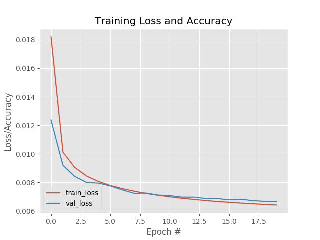
60000/60000 [==============================] - 73s 1ms/sample - loss: 0.0182 - val_loss: 0.0124
Epoch 2/20
60000/60000 [==============================] - 73s 1ms/sample - loss: 0.0101 - val_loss: 0.0092
Epoch 3/20
60000/60000 [==============================] - 73s 1ms/sample - loss: 0.0090 - val_loss: 0.0084
...
Epoch 18/20
60000/60000 [==============================] - 72s 1ms/sample - loss: 0.0065 - val_loss: 0.0067
Epoch 19/20
60000/60000 [==============================] - 73s 1ms/sample - loss: 0.0065 - val_loss: 0.0067
Epoch 20/20
60000/60000 [==============================] - 73s 1ms/sample - loss: 0.0064 - val_loss: 0.0067
[INFO] making predictions...
[INFO] saving autoencoder...

On my 3Ghz Intel Xeon W processor, the entire training process took ~24 minutes.

Looking at the plot in Figure 2, we can see that the training process was stable with no signs of overfitting:

Furthermore, the following reconstruction plot shows that our autoencoder is doing a fantastic job of reconstructing our input digits.

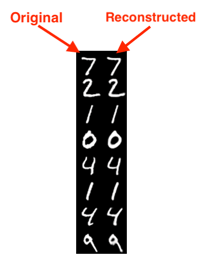
The fact that our autoencoder is doing such a good job also implies that our latent-space representation vectors are doing a good job compressing, quantifying, and representing the input image — having such a representation is a requirement when building an image retrieval system.

If the feature vectors cannot capture and quantify the contents of the image, then there is no way that the CBIR system will be able to return relevant images.

If you find that your autoencoder is failing to properly reconstruct your images, then it’s unlikely your autoencoder will perform well for image retrieval.

Take the proper care to train an accurate autoencoder — doing so will help ensure your image retrieval system returns similar images.

Implementing image indexer using the trained autoencoder

With our autoencoder successfully trained (Phase #1), we can move on to the feature extraction/indexing phase of the image retrieval pipeline (Phase #2).

This phase, at a bare minimum, requires us to use our trained autoencoder (specifically the “encoder” portion) to accept an input image, perform a forward pass, and then take the output of the encoder portion of the network to generate our index of feature vectors. These feature vectors are meant to quantify the contents of each image.

Optionally, we may also use specialized data structures such as VP-Trees and Random Projection Trees to improve the query speed of our image retrieval system.

Open up the index_images.py file in your directory structure and we’ll get started:

# import the necessary packages
from tensorflow.keras.models import Model
from tensorflow.keras.models import load_model
from tensorflow.keras.datasets import mnist
import numpy as np
import argparse
import pickle

# construct the argument parse and parse the arguments
ap = argparse.ArgumentParser()
ap.add_argument("-m", "--model", type=str, required=True,
	help="path to trained autoencoder")
ap.add_argument("-i", "--index", type=str, required=True,
	help="path to output features index file")
args = vars(ap.parse_args())

We begin with imports. Our tf.keras imports include (1) Model so we can construct our encoder, (2) load_model so we can load our autoencoder model we trained in the previous step, and (3) our mnist dataset. Our feature vector index will be serialized as a Python pickle file.

We have two required command line arguments:

• --model: The trained autoencoder input path from the previous step
• --index: The path to the output features index file in .pickle format

From here, we’ll load and preprocess our MNIST digit data:

# load the MNIST dataset
print("[INFO] loading MNIST training split...")
((trainX, _), (testX, _)) = mnist.load_data()

# add a channel dimension to every image in the training split, then
# scale the pixel intensities to the range [0, 1]
trainX = np.expand_dims(trainX, axis=-1)
trainX = trainX.astype("float32") / 255.0

Notice that the preprocessing steps are identical to that of our training procedure.

We’ll then load our autoencoder:

# load our autoencoder from disk
print("[INFO] loading autoencoder model...")
autoencoder = load_model(args["model"])

# create the encoder model which consists of *just* the encoder
# portion of the autoencoder
encoder = Model(inputs=autoencoder.input,
	outputs=autoencoder.get_layer("encoded").output)

# quantify the contents of our input images using the encoder
print("[INFO] encoding images...")
features = encoder.predict(trainX)

Line 28 loads our autoencoder (trained in the previous step) from disk.

Then, using the autoencoder’s input, we create a Model while only accessing the encoder portion of the network (i.e., the latent-space feature vector) as the output (Lines 32 and 33).

We then pass the MNIST digit image data through the encoder to compute our feature vectors (features) on Line 37.

Finally, we construct a dictionary map of our feature data:

# construct a dictionary that maps the index of the MNIST training
# image to its corresponding latent-space representation
indexes = list(range(0, trainX.shape[0]))
data = {"indexes": indexes, "features": features}

# write the data dictionary to disk
print("[INFO] saving index...")
f = open(args["index"], "wb")
f.write(pickle.dumps(data))
f.close()

Line 42 builds a data dictionary consisting of two components:

• indexes: Integer indices of each MNIST digit image in the dataset
• features: The corresponding feature vector for each image in the dataset

To close out, Lines 46-48 serialize the data to disk in Python’s pickle format.

Indexing our image dataset for image retrieval

We are now ready to quantify our image dataset using the autoencoder, specifically using the latent-space output of the encoder portion of the network.

To quantify our image dataset using the trained autoencoder, make sure you use the “Downloads” section of this tutorial to download the source code and pre-trained model.

From there, open up a terminal and execute the following command:

$ python index_images.py --model output/autoencoder.h5 \
	--index output/index.pickle
[INFO] loading MNIST training split...
[INFO] loading autoencoder model...
[INFO] encoding images...
[INFO] saving index...

If you check the contents of your output directory, you should now see your index.pickle file:

$ ls output/*.pickle
output/index.pickle

Implementing the image search and retrieval script using Keras and TensorFlow

Our final script, our image searcher, puts all the pieces together and allows us to complete our autoencoder image retrieval project (Phase #3). Again, we’ll be using Keras and TensorFlow for this implementation.

Open up the search.py script, and insert the following contents:

# import the necessary packages
from tensorflow.keras.models import Model
from tensorflow.keras.models import load_model
from tensorflow.keras.datasets import mnist
from imutils import build_montages
import numpy as np
import argparse
import pickle
import cv2

As you can see, this script needs the same tf.keras imports as our indexer. Additionally, we’ll use my build_montages convenience script in my imutils package to display our autoencoder CBIR results.

Let’s define a function to compute the similarity between two feature vectors:

def euclidean(a, b):
	# compute and return the euclidean distance between two vectors
	return np.linalg.norm(a - b)

Here we’re the Euclidean distance to calculate the similarity between two feature vectors, a and b.

There are multiple ways to compute distances — the cosine distance can be a good alternative for many CBIR applications. I also cover other distance algorithms inside the PyImageSearch Gurus course.

Next, we’ll define our searching function:

def perform_search(queryFeatures, index, maxResults=64):
	# initialize our list of results
	results = []

	# loop over our index
	for i in range(0, len(index["features"])):
		# compute the euclidean distance between our query features
		# and the features for the current image in our index, then
		# update our results list with a 2-tuple consisting of the
		# computed distance and the index of the image
		d = euclidean(queryFeatures, index["features"][i])
		results.append((d, i))

	# sort the results and grab the top ones
	results = sorted(results)[:maxResults]

	# return the list of results
	return results

Our perform_search function is responsible for comparing all feature vectors for similarity and returning the results.

This function accepts both the queryFeatures, a feature vector for the query image, and the index of all features to search through.

Our results will contain the top maxResults (in our case 64 is the default but we will soon override it to 225).

Line 17 initializes our list of results, which Lines 20-20 then populate. Here, we loop over all entries in our index, computing the Euclidean distance between our queryFeatures and the current feature vector in the index.

When it comes to the distance:

• The smaller the distance, the more similar the two images are
• The larger the distance, the less similar they are

We sort and grab the top results such that images that are more similar to the query are at the front of the list via Line 29.

Finally, we return the the search results to the calling function (Line 32).

With both our distance metric and searching utility defined, we’re now ready to parse command line arguments:

# construct the argument parse and parse the arguments
ap = argparse.ArgumentParser()
ap.add_argument("-m", "--model", type=str, required=True,
	help="path to trained autoencoder")
ap.add_argument("-i", "--index", type=str, required=True,
	help="path to features index file")
ap.add_argument("-s", "--sample", type=int, default=10,
	help="# of testing queries to perform")
args = vars(ap.parse_args())

Our script accepts three command line arguments:

• --model: The path to the trained autoencoder from the “Training the autoencoder” section
• --index: Our index of features to search through (i.e., the serialized index from the “Indexing our image dataset for image retrieval” section)
• --sample: The number of testing queries to perform with a default of 10

Now, let’s load and preprocess our digit data:

# load the MNIST dataset
print("[INFO] loading MNIST dataset...")
((trainX, _), (testX, _)) = mnist.load_data()

# add a channel dimension to every image in the dataset, then scale
# the pixel intensities to the range [0, 1]
trainX = np.expand_dims(trainX, axis=-1)
testX = np.expand_dims(testX, axis=-1)
trainX = trainX.astype("float32") / 255.0
testX = testX.astype("float32") / 255.0

And then we’ll load our autoencoder and index:

# load the autoencoder model and index from disk
print("[INFO] loading autoencoder and index...")
autoencoder = load_model(args["model"])
index = pickle.loads(open(args["index"], "rb").read())

# create the encoder model which consists of *just* the encoder
# portion of the autoencoder
encoder = Model(inputs=autoencoder.input,
	outputs=autoencoder.get_layer("encoded").output)

# quantify the contents of our input testing images using the encoder
print("[INFO] encoding testing images...")
features = encoder.predict(testX)

Here, Line 57 loads our trained autoencoder from disk, while Line 58 loads our pickled index from disk.

We then build a Model that will accept our images as an input and the output of our encoder layer (i.e., feature vector) as our model’s output (Lines 62 and 63).

Given our encoder, Line 67 performs a forward-pass of our set of testing images through the network, generating a list of features to quantify them.

We’ll now take a random sample of images, marking them as queries:

# randomly sample a set of testing query image indexes
queryIdxs = list(range(0, testX.shape[0]))
queryIdxs = np.random.choice(queryIdxs, size=args["sample"],
	replace=False)

# loop over the testing indexes
for i in queryIdxs:
	# take the features for the current image, find all similar
	# images in our dataset, and then initialize our list of result
	# images
	queryFeatures = features[i]
	results = perform_search(queryFeatures, index, maxResults=225)
	images = []

	# loop over the results
	for (d, j) in results:
		# grab the result image, convert it back to the range
		# [0, 255], and then update the images list
		image = (trainX[j] * 255).astype("uint8")
		image = np.dstack([image] * 3)
		images.append(image)

	# display the query image
	query = (testX[i] * 255).astype("uint8")
	cv2.imshow("Query", query)

	# build a montage from the results and display it
	montage = build_montages(images, (28, 28), (15, 15))[0]
	cv2.imshow("Results", montage)
	cv2.waitKey(0)

Lines 70-72 sample a set of testing image indices, marking them as our search engine queries.

We then loop over the queries beginning on Line 75. Inside, we:

• Grab the queryFeatures, and perform the search (Lines 79 and 80)
• Initialize a list to hold our result images (Line 81)
• Loop over the results, scaling the image back to the range [0, 255], creating an RGB representation from the grayscale image for display, and then adding it to our images results (Lines 84-89)
• Display the query image in its own OpenCV window (Lines 92 and 93)
• Display a montage of search engine results (Lines 96 and 97)
• When the user presses a key, we repeat the process (Line 98) with a different query image; you should continue to press a key as you inspect results until all of our query samples have been searched

To recap our search searching script, first we loaded our autoencoder and index.

We then grabbed the encoder portion of the autoencoder and used it to quantify our images (i.e., create feature vectors).

From there, we created a sample of random query images to test our searching method which is based on the Euclidean distance computation. Smaller distances indicate similar images — the similar images will be shown first because our results are sorted (Line 29).

We searched our index for each query showing only a maximum of maxResults in each montage.

In the next section, we’ll get the chance to visually validate how our autoencoder-based search engine works.

Image retrieval results using autoencoders, Keras, and TensorFlow

We are now ready to see our autoencoder image retrieval system in action!

Start by making sure you have:

1. Used the “Downloads” section of this tutorial to download the source code
2. Executed the train_autoencoder.py file to train the convolutional autoencoder
3. Run the index_images.py to quantify each image in our dataset

From there, you can execute the search.py script to perform a search:

$ python search.py --model output/autoencoder.h5 \
	--index output/index.pickle
[INFO] loading MNIST dataset...
[INFO] loading autoencoder and index...
[INFO] encoding testing images...

Below is an example providing a query image containing the digit 9 (top) along with the search results from our autoencoder image retrieval system (bottom):

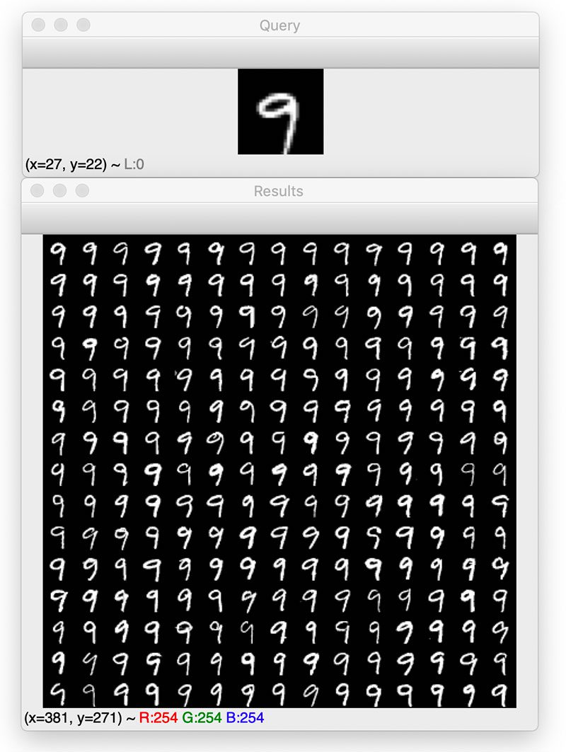
Here, you can see that our system has returned search results also containing nines.

Let’s now use a 2 as our query image:

Sure enough, our CBIR system returns digits containing twos, implying that latent-space representation has correctly quantified what a 2 looks like.

Here’s an example of using a 4 as a query image:

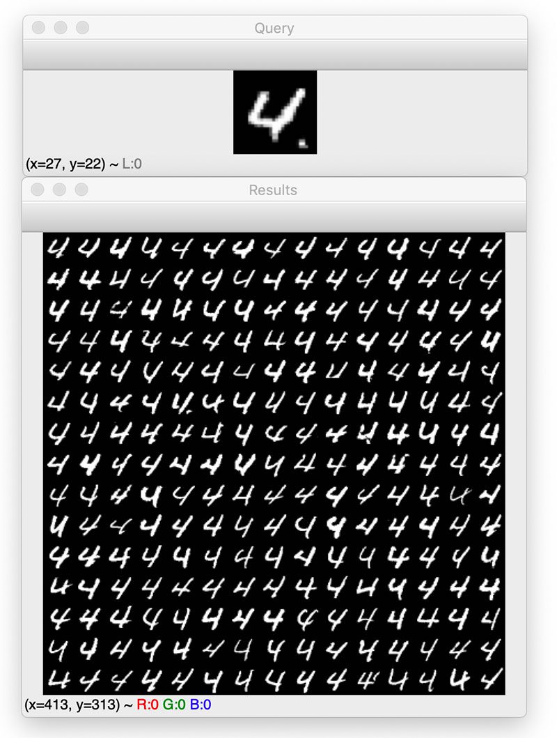
Again, our autoencoder image retrieval system returns all fours as the search results.

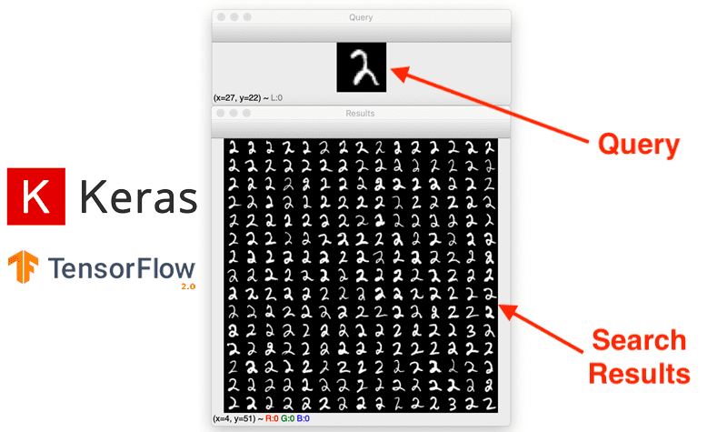
Let’s look at one final example, this time using a 0 as a query image:

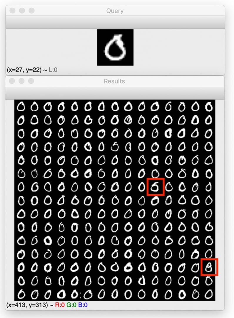
This result is more interesting — note the two highlighted results in the screenshot.

The first highlighted result is likely a 5, but the tail of the five seems to be connecting to the middle part, creating a digit that looks like a cross between a 0 and an 8.

We then have what I think is an 8 near the bottom of the search results (also highlighted in red). Again, we can appreciate how our image retrieval system may see that 8 as visually similar to a 0.

Tips to improve autoencoder image retrieval accuracy and speed

In this tutorial, we performed image retrieval on the MNIST dataset to demonstrate how autoencoders can be used to build image search engines.

However, you will more than likely want to use your own image dataset rather than the MNIST dataset.

Swapping in your own dataset is as simple as replacing the MNIST dataset loader helper function with your own dataset loader — you can then train an autoencoder on your dataset.

However, make sure your autoencoder accuracy is sufficient.

If your autoencoder cannot reasonably reconstruct your input data, then:

1. The autoencoder is failing to capture the patterns in your dataset
2. The latent-space vector will not properly quantify your images
3. And without proper quantification, your image retrieval system will return irrelevant results

Therefore, nearly the entire accuracy of your CBIR system hinges on your autoencoder — take the time to ensure it is properly trained.

Once your autoencoder is performing well, you can then move on to optimizing the speed of your search procedure.

Secondly, you should also consider the scalability of your CBIR system.

Our implementation here is an example of a linear search with O(N) complexity, meaning that it will not scale well.

To improve the speed of the retrieval system, you should use Approximate Nearest Neighbor algorithms and specialized data structures such as VP-Trees, Random Projection trees, etc., which can reduce the computational complexity to O(log N).

To learn more about these techniques, refer to my article on Building an Image Hashing Search Engine with VP-Trees and OpenCV.

What’s next?

If you want to increase your computer vision knowledge, then look no further than the PyImageSearch Gurus course and community.

Inside the course you’ll find:

• An actionable, real-world course on OpenCV and computer vision. Each lesson in PyImageSearch Gurus is taught in the same trademark, hands-on, easy-to-understand PyImageSearch style that you know and love
• The most comprehensive computer vision education online today. The PyImageSearch Gurus course covers 13 modules broken out into 168 lessons, with over 2,161 pages of content. You won’t find a more detailed computer vision course anywhere else online; I guarantee it
• A community of like-minded developers, researchers, and students just like you, who are eager to learn computer vision and level-up their skills

The course covers breadth and depth in the following subject areas, giving you the skills to rise in the ranks at your institution or even to land that next job:

• Automatic License Plate Recognition (ANPR) — recognize license plates of vehicles, or apply the concepts to your own OCR project
• Face Detection and Recognition — recognize who’s entering/leaving your house, build a smart classroom attendance system, or identify who’s who in your collection of family portraits
• Image Search Engines also known as Content Based Image Retrieval (CBIR)
• Object Detection — and my 6-step framework to accomplish it
• Big Data methodologies — use Hadoop for executing image processing algorithms in parallel on large computing clusters
• Machine Learning and Deep Learning — learn just what you need to know to be dangerous in today’s AI age, and prime your pump for even more advanced deep learning inside my book, Deep Learning for Computer Vision with Python

If the course sounds interesting to you, I’d love to send you 10 free sample lessons and the entire course syllabus so you can get a feel for what the course has to offer. Just click the link below!

Master computer vision inside PyImageSearch Gurus!

Summary

In this tutorial, you learned how to use convolutional autoencoders for image retrieval using TensorFlow and Keras.

To create our image retrieval system, we:

1. Trained a convolutional autoencoder on our image dataset
2. Used the trained autoencoder to compute the latent-space representation of each image in our dataset — this representation serves as our feature vector that quantifies the contents of the image
3. Compared the feature vector from our query image to all feature vectors in our dataset using a distance function (in this case, the Euclidean distance, but cosine distance would also work well here). The smaller the distance between the vectors the more similar our images were.

We then sorted our results based on the computed distance and displayed our results to the user.

Autoencoders can be extremely useful for CBIR applications — the downside is that they require a lot of training data, which you may or may not have.

More advanced deep learning image retrieval systems rely on siamese networks and triplet loss to embed vectors for images such that more similar images lie closer together in a Euclidean space, while less similar images are farther away — I’ll be covering these types of network architectures and techniques at a future date.

To download the source code to this post (including the pre-trained autoencoder), just enter your email address in the form below!

The post Autoencoders for Content-based Image Retrieval with Keras and TensorFlow appeared first on PyImageSearch.